Lecture 20: Cannon’s Algorithm¶

Cannon’s algorithm¶

Let’s start with the block algorithm for matrix-matrix multiply. We first partition the matrix into blocks. Next we assign the block matrices to different ranks. Each owner rank who possesses the block matrix performs the computation.

We have three different matrix partitioning strategies: block partitioning, cyclic partitioning, and block cyclic partitioning.

Based on the above idea, we have Cannon’s algorithm for the distributed matrix-matrix product. First, we have a 2D decomposition of input matrices A and B, and output matrix C. Next, we move block matrices A and B to their starting positions/ranks by mapping the block matrix to the corresponding ranks. Now we are ready to do matrix-matrix product local to each rank. After each computation, we will shift the block matrices left as well as up in the rank/processor grid. Then we perform computation locally after we receive the new block matrices until all blocks have been touched. Finally, we move matrices A and B back to initial distribution.

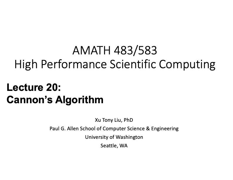
Below is an illustration of how each block matrix is being passed in the processor grid. Let’s start at step 0 after the first local computation. We shift the block matrices left in the rank/processor grid.

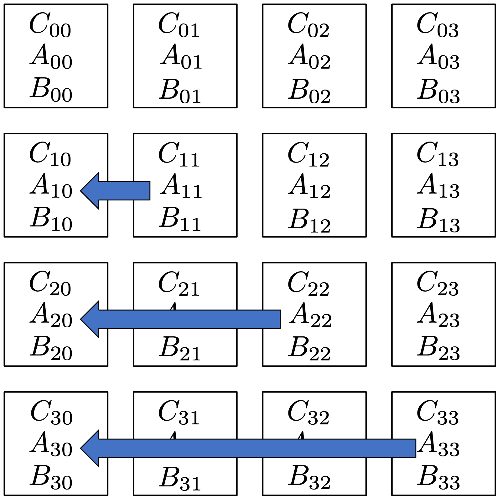
We end up with:

Next we shift the block matrices up in the rank/processor grid.

We end up with:

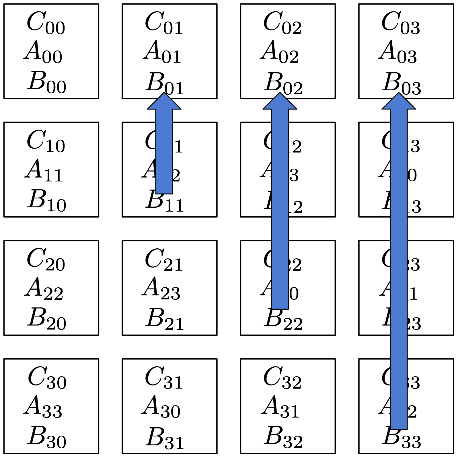
Let’s proceed to step 1. If we combine the shift left and up in one figure, this is how it looks like.

Based on this communication pattern, it is too painful for us to implement using basic MPI communicator. Luckily, we can create a Cartesian Communicator which topology information has been attached. Since we have a 2D processor grid, we can tell our Cartesian communicator about this 2D topology of ours. Next using the Cartcomm::Shift, and Cartcomm::Sendrecv_replace, we can shift our block matrix up and left easily. Similarly, once we finish the computation, we can use them to restore block matrices A and B to initial distribution.