Sparse vs Dense Computation (Or, How to be Faster while Being Slower)¶

Question: Why use sparse computation when dense computation is so much faster?¶

It is true that the rate at which dense computation can be done is much faster than for sparse computation. Dense matrix computation can often approach the peak floating point rate of a CPU (or GPU). Sparse matrix computations, on the other hand, tend to be memory bound. For example at the SC’19 student cluster competition, using the same hardware, the UW team achieved nearly 42 TFlop/sec on the High-Performance Linpack benchmark (dense) but only about 1 TFlop/sec on the High-Performance Conjugate Gradient benchmark (sparse). Why would you want to give up a factor of 40 in performance?

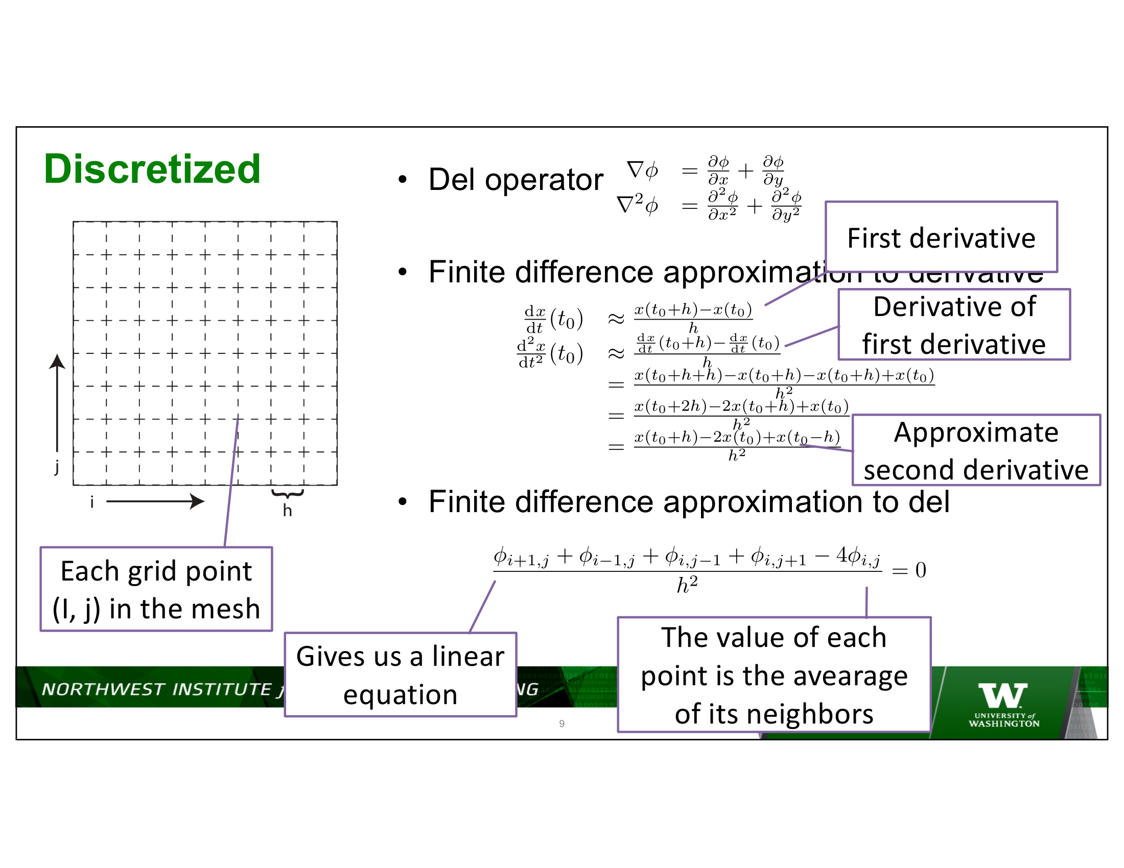
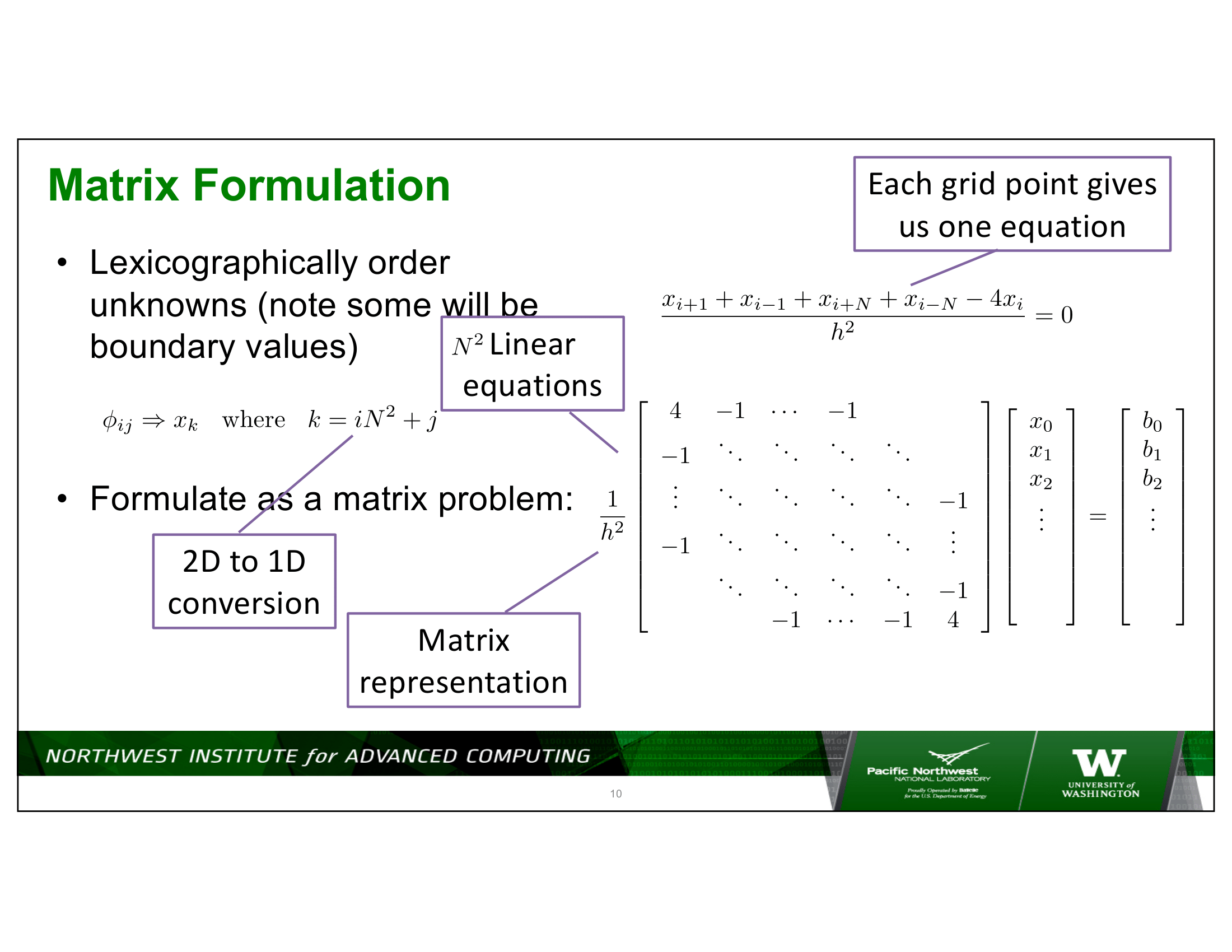
We discussed this a bit in lecture 9. Ultimately the question isn’t about how fast can work be done, but how fast can useful work be done. In many scientific computations, we are simulating systems of PDEs, which, when discretized, result in very sparse systems – meaning the matrix is almost completely full of zeros. And, in fact, as the systems being discretized get larger, the proportion of non-zero to zero elements becomes even smaller. (You can think of an entry in a matrix as meaning there is an interaction between two points in the discretized system – the universe is local – the only interactions are with nearby points.)

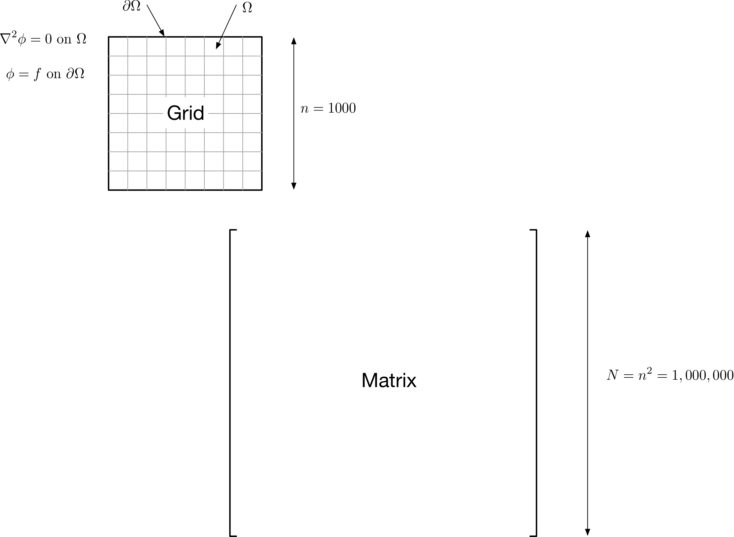
To put some numbers on this – consider a 2D discretization of Laplace’s equation on a square domain, with, say, 1,000 discretization indexes in each dimension – for a total of 1,000,000 points in the domain being discretized.

The following table is an example of the differences in compute times:

This is a very optimistic assessment of performance for the dense case. In reality, 8,000 GB cannot even be stored in a single computer system, much less computed on. Moreover, the rate of computation would be much lower for a problem of this size, which would also become memory bound (since this is matvec rather than mat-mat).

If you would like to try benchmarking this yourself, you can download sparse_vs_dense.cpp. It should work with the code from your midterm, with the exception of three functions you will have to add to amath583.cpp (and amath583.hpp) shown below. Note that this benchmark runs each test only once. For the sizes of problems that are possible with the dense computation, most of the sparse computations finish in less than a millisecond, whereas the dense computations rapidly grow in time.

// Declarations go in amath583.hpp
void piscetize(Matrix &A, size_t xpoints, size_t ypoints);
Vector mult(const Vector& x, const Matrix& A);
void mult(const Vector& x, const Matrix& A, Vector& y);

// Code goes in amath583.cpp
void piscetize(Matrix &A, size_t xpoints, size_t ypoints) {
  assert(A.num_rows() == A.num_cols());
  assert(xpoints * ypoints == A.num_rows());

  zeroize(A);

    for (size_t j = 0; j < xpoints; j++) {
    for (size_t k = 0; k < ypoints; k++) {
      size_t jrow = j * ypoints + k;

      if (j != 0) {
        size_t jcol = (j - 1) * ypoints + k;
        A(jrow, jcol) = -1.0;
      }
      if (k != 0) {
        size_t jcol = j * ypoints + (k - 1);
        A(jrow, jcol) = -1.0;
      }
      A(jrow, jrow) = 4.0;

      if (k != ypoints - 1) {
        size_t jcol = j * ypoints + (k + 1);
        A(jrow, jcol) = -1.0;
      }
      if (j != xpoints - 1) {
        size_t jcol = (j + 1) * ypoints + k;
        A(jrow, jcol) = -1.0;
      }
    }
  }
}

Vector mult(const Vector& x, const Matrix& A) {
  Vector y(A.num_rows());
  mult(x, A, y);
  return y;
}

void   mult(const Vector& x, const Matrix& A, Vector& y) {
  assert(y.num_rows() == A.num_rows());
  for (size_t j = 0; j < A.num_cols(); ++j) {
    for (size_t i = 0; i < A.num_rows(); ++i) {
      y(i) += A(j, i) * x(j);
    }
  }
}