Problem Set #1¶

Set Up Your Development Environment¶

For a number of reasons (some of which we discussed in lecture), the platform that supports most high-performance computing today is Linux with its associated terminal-based command-line tools. Although personal computers today have a different paradigm for interaction, a Linux environment can be fairly well approximated on Windows 10 and Mac OS X.

The particular development tools that will need to be in your development environment are the following (how to obtain and install them is described below).

• Visual Studio Code (latest available version)

• Docker (latest available version)

There will be additional packages to add for future assignments, but these will be sufficient for the next few assignments.

Install Visual Studio Code¶

You can search for Visual Studio Code with Google and download the installer from a site at Microsoft. Note that Visual Studio Code is not the same (at all) as Visual Studio, so be sure to search for Visual Studio Code and not just Visual Studio. Notice that

Customize Visual Studio Code¶

Once vscode is installed, you need to adjust a couple of settings. Right click on the gear icon in the lower left corner of vscode and select ``Command Palette’’. At the command palette prompt, type ``Terminal: Select Default Shell’’. You will get a drop down menu with three choices. Select ``Bash.’’

Now click on Terminal in the vscode menu bar and select ``New Terminal’’. A window will open in the bottom half of vscode. You should see a bash prompt there. Issue the command

$ cd

To go to your home directory. (The shell defaults to a different initial directory than your home.) You can also start a terminal with the ctrl+ \ key combination (control and back-tick together). The terminal should behave just like a bash shell that you start from the start menu.

Finally, in the left hand column there are some icons, the bottom of which are four square boxes (more or less). Click on that to bring up an extensions panel. The third (or so) entry should be C++ intellisense. Click to install that. There are a huge number of other extensions that you might want to browse and explore, but the most important one is C++ intellisense. If C++ intellisense is not the near the top of the list, you can search for it in the search bar at the top of that column.

(I suggest also installing live share and live share extensions to enable collaborative editing.)

Virtualization¶

Delivering software (and/or services) to others in our modern highly-interconnected and highly-heterogeneous world is a challenge. The connectivity makes it easy to actually deliver the bytes comprising the software, but the wide variety of operating systems (Windows, Mac OS X, Linux), there versions, and hardware platforms (x86, x86_64, ARM), makes actually running the software at the end point seems almost impossible. A modern application typically composes together numerous other software frameworks (windowing libraries, networking, etc) and relies on host operating system services.

One approach that is somewhat helpful in addressing this is to have a minimal set of standardized services that all environments are expected to provide. A program written to just use those services will run anywhere that those requirements are met. But we’ve already seen some of the limitations of that approach in this course – the standards aren’t really standard and restricting your program to a minimal set can be quite limiting.

One increasingly popular – and highly effective – approach is virtualition. The idea behind virtualization is insert a thin software layer on top of the actual local OS – and have that thin layer provide a generic and portable interface. For those of you running the Windows Subsystem for Linux – this is exactly what is happening. The Linux programs you are running in WSL aren’t ported or rewritten for Windows (or rewritten for WSL): they are the very same binaries that a native Linux installation would run.

There are some third-party virtualization systems (aka virtual machines) such as VMWare or VirtualBox that will let you run a complete OS inside of another OS. WSL isn’t quite that heavy-weight – the virtualization layer instead provides all of the services as if it wer a complete OS. A similar (but portable and third-party) light-weight system for virtualization is docker.

Install Docker¶

Detailed instructions on how to obtain, download, and install Docker can be found on the Docker web site. Some basic steps are provided below, but the instructions on the web site are definitive.

If your computer and operating system are sufficiently recent, you will be able to run Docker directly. Docker has the same requirements on Windows as for WSL: you will need Win 10 Pro and will need to enable virtualization.

Step by step instructions for downloading, installing, and verifying Docker can be found here.

Verify Your Docker Installation¶

Steps for verifying Docker are at Step 3 on this page. You should use Terminal.app (“Terminal”) on Mac OS X and PowerShell on Windows.

Install the AMATH583 Docker Image¶

In the verification steps on docs.docker.com, you executed some images with the “docker run” command. As mentioned on the site, this first pulled the image to be executed from the docker site and then executed it. For this course we have created several custom images with tools (and applications) required to carry out certain tasks and assignments.

To download the basic image to your local machine, issue the following command in your terminal:

$ docker pull amath583/sp21:amd64

The image is fairly large (around 4GB) so the download will take some time, depending on the speed of your network connection. Once your download is finished, issue the following command in your terminal to verify:

$ docker image ls
 REPOSITORY                 TAG       IMAGE ID       CREATED         SIZE
 amath583/sp21              amd64     4beebecadd0d   19 minutes ago  3.9GB

This command will list all the installed docker images on your machine. Notice that the “REPOSITORY” list the image name “amath583/sp21”, and the “TAG” is “amd64”. Once we have image installed, we can proceed to next step.

$ docker pull amath583/sp21:arm64

$ docker image ls
REPOSITORY                 TAG       IMAGE ID       CREATED         SIZE
amath583/sp21              arm64     30d51c680610   11 hours ago    3.47GB

Other images created for this course include:

• amath583/base : Ubuntu installation with clang compiler

• amath583/ps3 : base image plus python and matplotlib

• amath583/ert : an application image for generating a one-core roofline plot for your computer

• amath583/bandwidth : an application image for generating a bandwidth plot for your computer

• amath583/bandwidth.noavx : same as above, but without advanced CPU instructions (that might not be supported on all platforms)

• amath583/openmp : base image plus support for OpenMP

• amath-583-ert.openmp : an application image for generating a multiple-core roofline plot for your computer

Connect to Your Local Workspace¶

There is an important feature to remember about running an image in a Docker container: Whatever you do in the container is not permanently saved. If you do your work in the container and save some files in the container, the next time you start the container, those files will be gone.

Fortunately, Docker provides a mechanism to share files between running containers and the host file system (your folders and files). To do that we use a command line option with Docker to map a folder in your home directory (the folder that you were asked to make above) to a directory in the running container.

Now we are ready to run the amath583/sp21 image in a Docker container. Remember the following command (write it down, save it to a note file, etc) as you will be running it every time you need to work on programming assignments for this course.

For Mac OS X (assuming /Users/<your-id>/amath583work is where your amath583 assignments are):

$ docker run -it -v /Users/<your-id>/amath583work:/home/amath583/work amath583/sp21:amd64

For Windows (assuming C:\Users\<your-netid>\amath583\work is where your amath583 assignments are):

$ docker run -it -v C:\\Users\\<your-netid>\\amath583\\work:/home/amath583/work amath583/sp21:amd64

$ docker run -it -v /Users/<your-id>/amath583/work:/home/amath583/work:Z amath583/sp21:amd64

amath583@892dae99e90b:/$

bin   dev  home  lib64  mnt  proc  run   srv  tmp  var
boot  etc  lib   media  opt  root  sbin  sys  usr

amath583@892dae99e90b:~$

tmp  work

$ cd work
$ ls

$ cd work   # change into your work directory
$ touch hello
$ ls

$ cd
$ touch work/goodbye
$ touch tmp/goodbye
$ ls work
$ ls tmp

$ cd
$ ls work
$ ls tmp

$ docker cp /home/amath583/work/hello 892dae99e90b:/home/amath583/work/

$ docker cp 892dae99e90b:/home/amath583/work/hello /home/amath583/work/

Docker and Visual Studio Code¶

As we have already seen in the course, one powerful feature of VS Code is that it can run an integrated terminal (described here.)

Since VS Code can be extended so flexibly, for situations that might require it, we can in fact configure VS Code to use a Docker image as the shell for the integrated terminal. This requires a few steps in manually modifying the configuration of VS Code, described in the following.

First, start up VS Code. In the lower left hand corner you will see the universal sign for settings (a gear). Click on that and choose “Settings” from the menu.

This will open up an editor window where you can edit (in JSON format) any of the hundreds and hundreds of settings in VS Code. We just want to edit two.

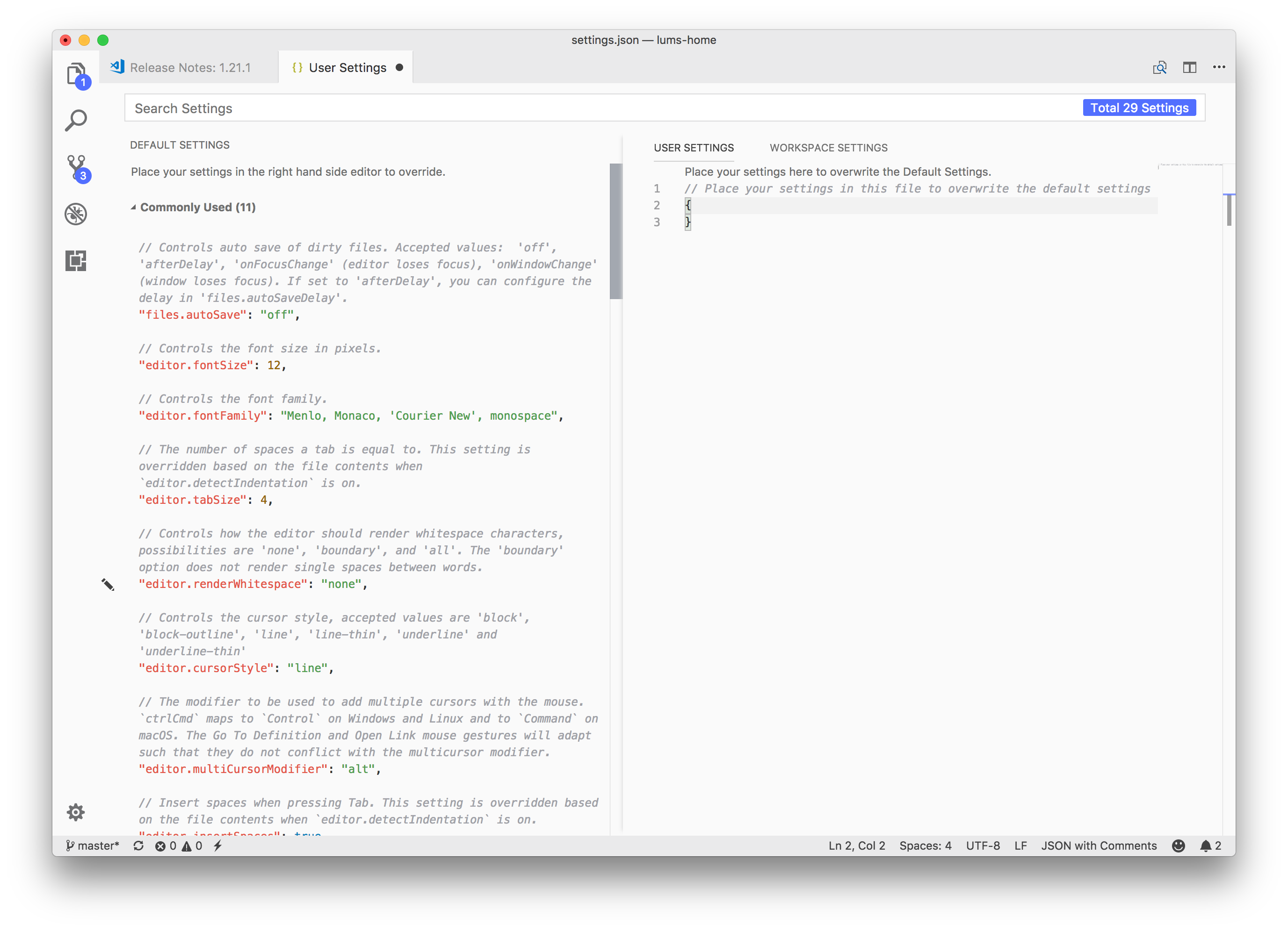
The setting we are modifying is “terminal.integrated.profiles” (search “terminal.integrated.profiles” in the search box). Click on “Edit in settings.json”. This will open the settings file as a json file.

Mac OS Instructions¶

For Mac OS, enter the code as shown into the editor window, between the curly braces. You should do this in the “user settings” tab rather than workspace settings.

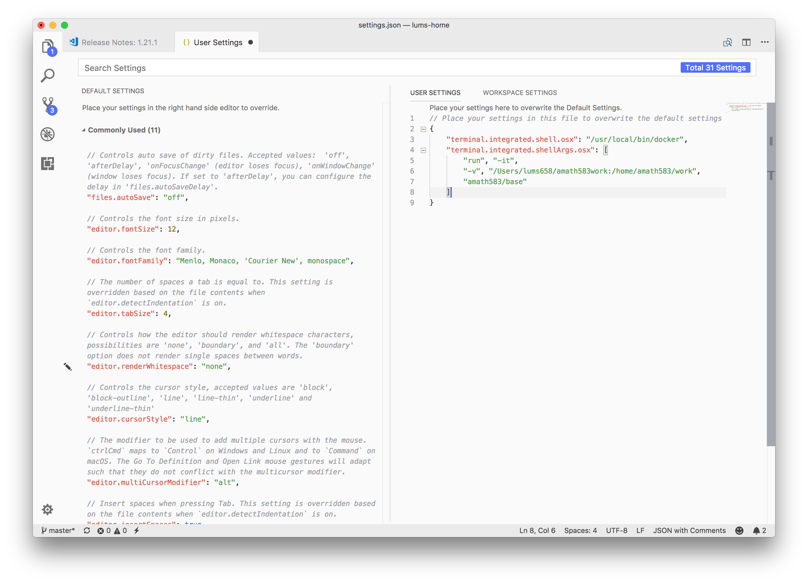
If you would like to cut and paste – use the below:

"terminal.integrated.profiles.osx": {
  "docker": {
    "path": "/usr/local/bin/docker",
    "args": [
      "run",
      "-it",
      "-v",
      "/Users/<yourid>/amath583/work:/home/amath583/work",
      "amath583/sp21:amd64"
    ]
  }
},

Replace \(\langle\) yourid \(\rangle\) with your user id on your computer – /Users/<yourid>/amath583/work should be the path to where you do your work on your computer – and where you want docker and your host OS to link.

Finally, start the integrated terminal either through the menu (View \(\rightarrow\) Integrated Terminal) or with the keyboard shortcut ^~ (control-tilde). Remember to select “docker” profile instead of others in order to run docker container in VSCode’s integrated terminal.

"terminal.integrated.profiles.windows": {
  "docker" : {
    "path": "docker.exe",
    "args": [
      "run",
      "-it",
      "-v",
      "C:\\Users\\<yourid>\\amath583\\work:/home/amath583/work",
      "amath583/sp21:amd64"
    ]
  }
},

The Shell¶

The program that runs when you start bash is the “bash” shell. A shell is a program that can execute other programs as well as its own scripts. When run in interactive mode, the shell prints a prompt to the screen and waits for user input. The user enters text and when the user hits return, the shell attempts to execute the command and then again prompts the user for input.

Our development environment has documentation available for most of the commands that you will be using. These are generally comprehensive – which is good – but sometimes it can be difficult to locate exactly what you are looking for. In those cases your favorite search engine (and/or Piazza) can be your friend.

Three commands that are essential for navigating a Linux filesystem are cd, pwd, and ls, which change directory, print the working directory, and list the contents of the current directory, respectively. The ls command has a number of options that you can use with it to control what is displayed and how. The linux filesystem is basically a tree of directories (folders), each of which can contain files and other directories (sub-directories). The top-level directory is called “/”. The directories with the operating system and the linux home directories are subdirectories under “/”. When you ran ls above, you listed the contents of your “home” directory (your working directory), which in the case of Windows were the “dot” files.

To change to a different directory, use the cd (change directory) command. If you issue cd without any arguments you will change to your home directory, which we established above. If you provide an argument to cd the shell will attempt to change your working directory to the indicated path (a path is a sequence of directories, possibly ending in a file). There are two types of paths that you can supply – absolute or relative. An absolute path begins at the root, i.e., / while a relative path begins with the name of a subdirectory in the current directory. Finally, you can determine which is the current working directory for the shell by issuing the command pwd (print working directory).

For example, if your current working directory is / then when you issue the command pwd it will print /. The following two commands are equivalent (one is relative, one is absolute):

$ cd /
$ cd tmp

is equivalent to

$ cd /tmp

Note that ls can also take arguments, again an absolute or a relative path:

$ ls tmp
$ ls /tmp

There are two special subdirectories in every directory: . (dot) and .. (dotdot). Dot is the name of the current directory. If you issue ls . you will get the contents of the current directory. Dotdot is the name of the parent directory (recall that the filesystem is a tree – each directory has a unique parent, up to “/”). Try out . and .. with the “ls” and “cd” commands.

The Shell from vscode¶

Regardless of whether you are using Windows, Mac OS, or Linux, it can be quite helpful to access a shell from vscode (per the instructions above). A typical workflow is edit-compile-run-debug. Using a shell from within vscode allows you to issue the commands to compile and run from the same environment as you are editing without having to switch windows. (Like many IDEs, vscode also allows you to compile, run, and debug from within the editor.)

Help and Documentation¶

Your installation contains documentation for the packages that were installed with it. The typical Linux way of viewing the documentation is the man (manual) command. To view documentation of a particular command, invoke man with the name of the command as an argument. For example

$ man ls

will display the documentation for the ls command. Many commands that you issue at the command prompt are executable programs stored in the filesystem (usually in /bin, /usr/bin, or /usr/local/bin). However, some commands are built-in shell commands – cd for example is a built-in command. To find out information about built-in shell commands, use “help” (which is also built-in). Note that there is a difference between “man” and “help”.

Explore¶

Now, take a few minutes to move around the directory structure in your environment. Some directories to look at might be /usr/bin or /usr/include. Two more commands that you might find handy are cat and more.

Creating and Editing Files¶

For the rest of this course you will be creating and editing source code files – each assignment should go in a separate folder (subdirectory). When using visual studio code you can work with a single folder at a time – it will only show you the contents of the currently open folder. Use the File->Open… menu option and select the specific folder you want to work with. You can open any folder you like and the editor will show you all of the folders and files underneath it. I recommend just opening the folder associated with the current problem set. When you close and reopen vscode it will keep a record of which folder you had open and bring you back to that. When you want to work on the next assignment, close the current folder and open the next.

Hello World!¶

In your working directory, create a sub-directory named ps1. Open that folder with vscode and create a file called hello.cpp with the following contents:

#include <iostream>

int main() {

  std::cout << "Hello World" << std::endl;

  return 0;
}

Save the file and use cat or more to verify its contents. (What does the less command do?)

Now, execute the following commands:

$ c++ hello.cpp
$ ./a.out

std::vector¶

The C++ standard library contains a number of basic data structures – lists, arrays, hash maps, etc. The data structure that will be our workhorse (though we will be wrapping it up in other data structures) is std::vector.

The std::vector is a generic container – meaning it can hold data of any type. However, as we mentioned in lecture, C++ is a compiled and strongly typed language. The generic container can hold any type – but we have to specify the type to the compiler. To create a vector of integers with ten elements, we would use the statement

std::vector<int> x(10);

The type that the vector is holding is specified in the angle brackets; the size of the vector we are creating has 10 elements.

Elements of a std::vector are accessed with square brackets:

int a = x[3];

assigns the value of the element at index 3 to the variable a.

We can loop through a vector from beginning to end using the square bracket notation:

for (int i = 0; i < 10; ++i) {
    x[i] = 2 * i;
}

This loop specifies to assign values 0 to 9 (nine) to i and assign 2*i to each x[i]. Another consequence of zero-based indexing is that the final element in an array is location size - 1.

Now, if you aren’t familiar with it, it might seem that zero-based indexing is going to require you to always be adding and subtracting 1 from index values. In fact, zero-based indexing is the natural indexing for computer programming and you will rarely, if ever, see code that is accessing arrays having to add and subtract 1s from index values. On the other hand, you have probably experienced having to do this when programming with Matlab (for instance).

A very common error in C++ programming is to exceed the bounds of an array when reading or writing date from or to it. Unlike interpreted languages, these bounds are not checked when the program is running. However, the above for loop is an extremely common pattern. We begin at the beginning of the vector and loop to the end. The index variable i starts at 0 and the loop continues as long as i is less than 10 (the number of elements we want to loop over). The ++i statement indicates that the value of i should be incremented by one at the end of each loop.

A Non-Trivial First Program¶

Now, with all of those preliminaries out of the way…

The program I want you to write for this assignment is to plot the value of \(\cos(x)\) with 1024 points for x from 0 to \(4\pi\), inclusive. Important: I want you to include \(\cos(4\pi)\) as the final value, not “\(\cos\) of almost \(4\pi\)”.

(Hint: be thoughtful about how you index into the std::vector.)

A basic skeleton of the program to do this plotting is

 1#include <cmath>
 2#include <iostream>
 3#define WITHOUT_NUMPY
 4#include "matplotlibcpp.h"
 5
 6namespace plt = matplotlibcpp;
 7
 8int main () {
 9  double pi = std::acos(-1.0);  // C++ does not mandate a value for pi
10
11  plt::figure_size(1280, 960);  // Initialize a 1280 X 960 figure
12
13  std::vector<double> x(1024);  // Create two vectors
14  std::vector<double> y(1024);
15
16  // Fill in x with values from 0 to 4*pi (equally spaced)
17  double N = 4.0;
18  for (size_t i = 0; i < 1024; ++i) {
19    // WRITE ME
20  }
21
22  // Fill in y with cos of x
23  for (size_t i = 0; i < 1024; ++i) {
24    // WRITE ME
25  }
26
27  // Check that the last value of x has the right value
28  if (std::abs(x[1023] - N * pi) < 1.0e-12) {
29    std::cout << "Pass" << std::endl;
30  } else {
31    std::cout << "Fail" << " " << std::abs(x[1023] - N * pi) << std::endl;
32  }
33
34  // Make the plot and save it to a file
35  plt::plot(x, y);
36  plt::save("cosx.png");
37
38  return 0;
39}

Download cos4pi.cpp and copy it to your ps1 work directory (with the filename cos4pi.cpp).

You will also need the file matplotlibcpp.h which you can download here: matplotlibcpp.h

This file is a C++ header file to do plotting and image manipulation (we will be using it several times in this course).

There are two places in the file cos4pi.cpp that say “WRITE ME”. The first is within a loop that increments a value of i (which value you can use within the loop) from 0 to its limit (what is the limit?). Replace the “Write Me” with a statement that fills in the vector x with the values from 0 to 4*pi (equally spaced).You will need to scale the value of i by some constant value to get the equally-spaced points and the correct final value.

In the second “Write Me” you should fills in the vector y with \(\cos\) of x such that the last value computed will be exactly \(\cos(4\pi)\) (exactly, that is, within floating point precision).

Once we fill the vector of x and y, we call the function plt::plot with the data you want to plot (the vector x and y). plt::plot is a function that will plot the values it is passed, then we save those values to an image file “cosx.png” using plt::save.

Each “WRITE ME” should only require a single line of C++ code.

To compile your program, use the following command. You can just cut and paste this into your shell window; we will be looking at how to automate this process during lectures 3 and 4.

$ c++ -std=c++11 cos4pi.cpp -I/usr/include/python3.8 -lpython3.8

You can then execute your program using this command

$ ./a.out

This will create a file cosx.png in your work directory. You can view it with the image viewing program of your choice.

(Hint: your plot should look like one of the alphabet letters. If not, you are not doing it right.)

Written Exercises¶

Create a text file called ex1.txt in your ps1 folder. In that file, copy the following questions. Start your answers on a new line after each question and leave a blank line between the end of your answer and the next question.

1. How would you specify the name of an output file when you use the compiler if you wanted the executable to have a name other than a.out?

2. What happens if you type

$ a.out

instead of

$ ./a.out

to run your program? What is the difference (operationally) between the two statements?

3. What does clang print when you run

$ c++ --version

(TL: note two dashes before version.)

4. In the example program, the i variable is said to be size_t. What is a size_t?

5. In cosx.png, which alphabet letter does the shape look like?

6. (AMATH 583 only). What do the -I and -l flags do in the command we used to build a.out? (TL: In case the fonts make the two flags look the same, one is lower-case “L” (ell) and one is upper-case “I” (eye).)