Lecture 7: Optimizing for CPUs and Hierarchial Memory¶

Benchmarking¶

In this unit we are going to systematically develop and apply optimizations to the (dense) matrix-matrix product algorithm, with the goal of maximizing locality and thereby maximizing performance. We measure performance of matrix-matrix product in GFlop/s (billions of floating point operations per second).

Using the Matrix class we developed last tiem, the basic matrix-matrix multiply looks like this:

void multiply(const Matrix& A, const Matrix&B, Matrix&C) {
  for (size_t i = 0; i < A.num_rows(); ++i) {
    for (size_t j = 0; j < B.num_cols(); ++j) {
      for (size_t k = 0; k < A.num_cols(); ++k) {
        C(i,j) += A(i,k) * B(k,j);
      }
    }
  }
}

We compute GFlop/s by counting the number of floating point operations and dividing by the time taken (using a timer routine around the multiply operation. For \(A\in\Real^{M\times K}, B\in\Real^{K\times N}\), and \(C\in\Real^{M\times N}\), there are \(2\time K\times M\times N\). (You can easily verify this by noting the outer loop of multiply loops \(M\) times, the middle loop iterates \(N\) times and the inner loop iterates \(K\) times – and there are two floating point operations in the inner loop: one multiply and one add.) If we assume \(K\), \(M\), and \(N\) are the same order, then we can succinctly say the order of complexity of matrix-matrix product is cubic in the size of the problem, i.e., that it is \(O(N^3)\).

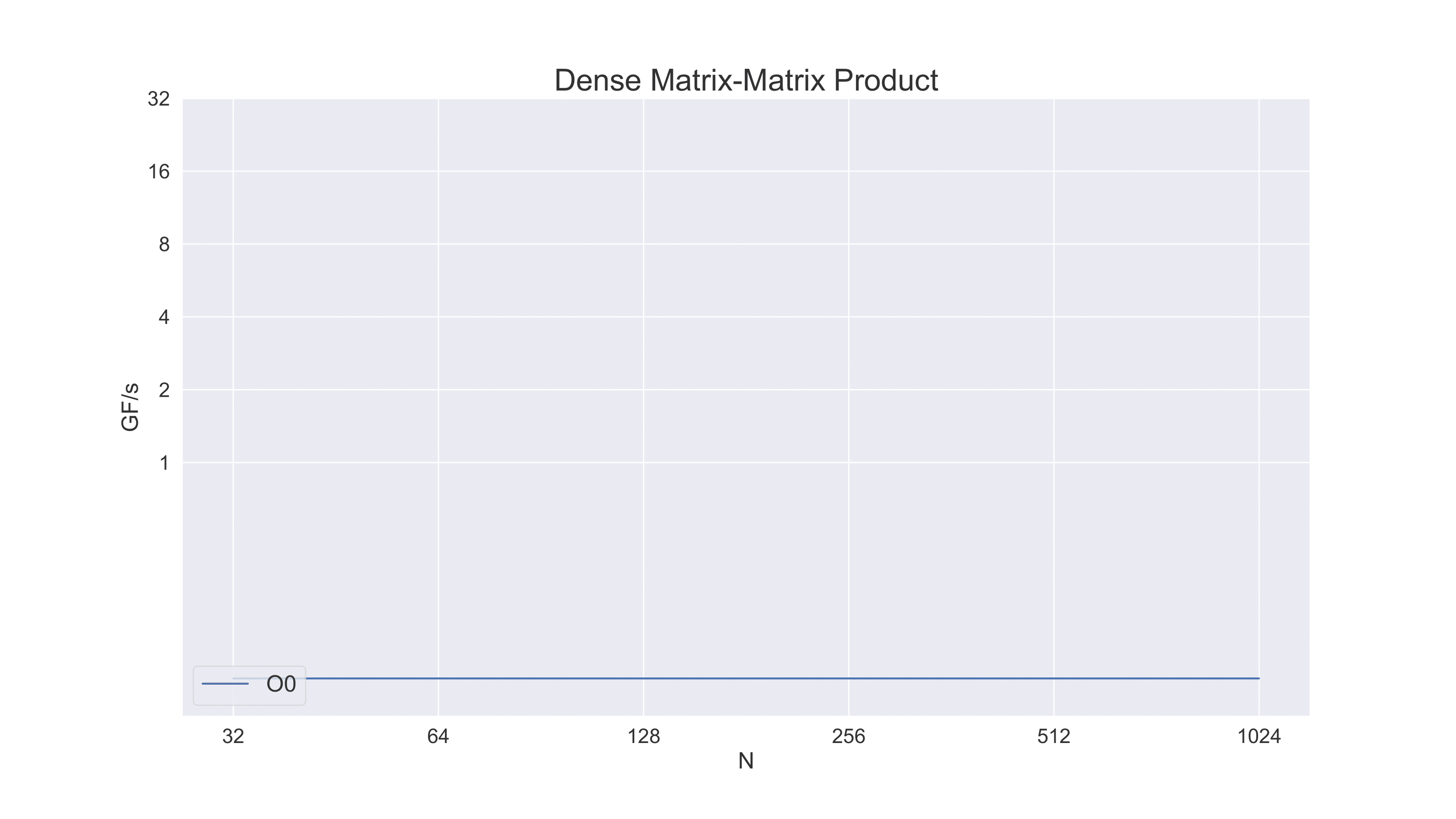
Below is the result of timing matrix multiply in its basic form on an Apple Macbook Pro — and using the compiler in its basic form. The level of performance is about 0.12 GFlop/s. Although that may have been considered high performance some decades ago, it is in fact just a small fraction of what we will ultimately be able to achieve.

One immediate (and substantial) improvement that we can make is to compile the benchmrking program with optimization enabled. In this case (and for the rest of the plots below) we use -Ofast -march=native. This enables maximum optimization as well as use of performance-oriented architecture features of the actual processor being used for compilation. (By default the compiler must assume a lowest common set of features.)

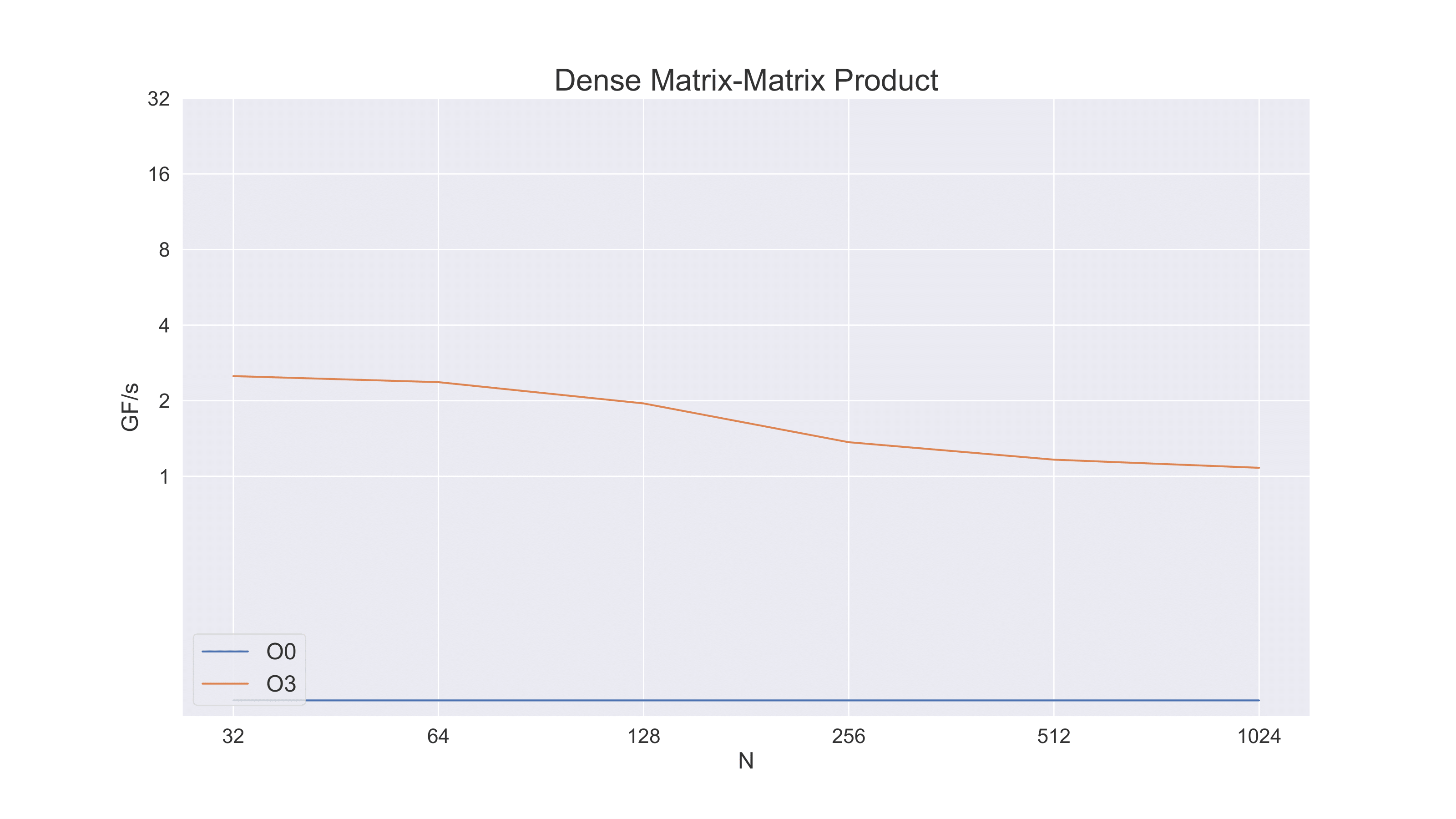
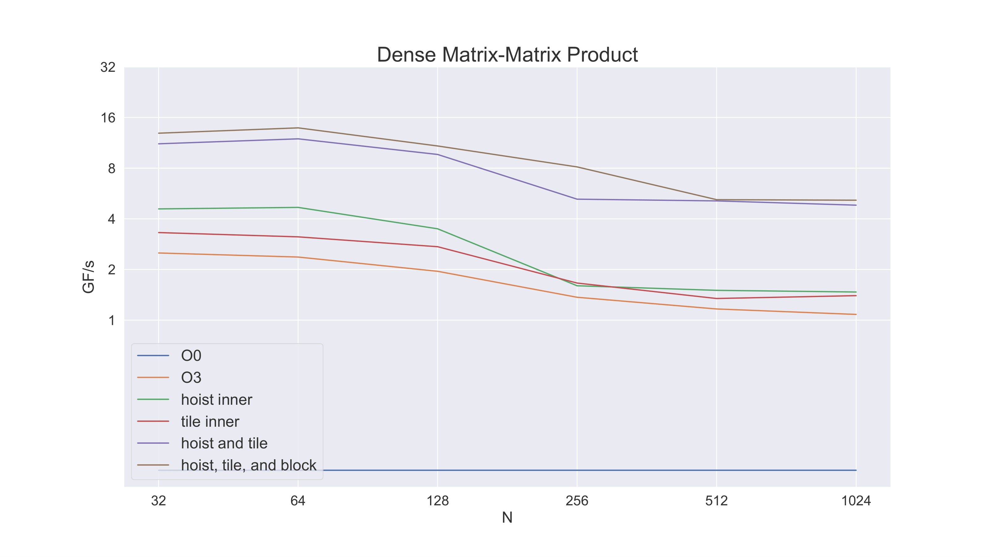
In this plot we are plotting performance as a function of problem size. (We are using \(M=N=K\) for our matrices and putting the value of \(N\) on the x axis.) The performance starts at around 2.5 GFlop/s but then degrades to about 1.0 GFlop/s. This is due to the problem not yet exploiting much locality. Larger problems do not naturally fit as well into cache and so the performance degrades as the problem gets larger. In fact, we would expect the performance at larger problem sizes to be dominated by memory bandwidth rather than CPU performance. In a future unit we will formalize this somewhat with the “roofline model.”

Now, we can observe that at each trip through the inner loop that C(i,j) is read and written and that A(i,k) and B(k,j) are read. Thus there are a total of six operations in each trip through the inner loop – two floating point operations and four memory operations. Expected efficiency is therefore about 1/3.

A consequence of exploiting locality is reuse. If we look at the inner loop of the multiply routine, we see that C(i,j) is being read and written – even though it does not depend on k. We can therefore hoist that variable out of the inner loop:

void multiply(const Matrix& A, const Matrix&B, Matrix&C) {
  for (size_t i = 0; i < A.num_rows(); ++i) {
    for (size_t j = 0; j < B.num_cols(); ++j) {
      double t = C(i,j);
      for (size_t k = 0; k < A.num_cols(); ++k) {
        t += A(i,k) * B(k,j);
      }
      C(i,j) = t;
    }
  }
}

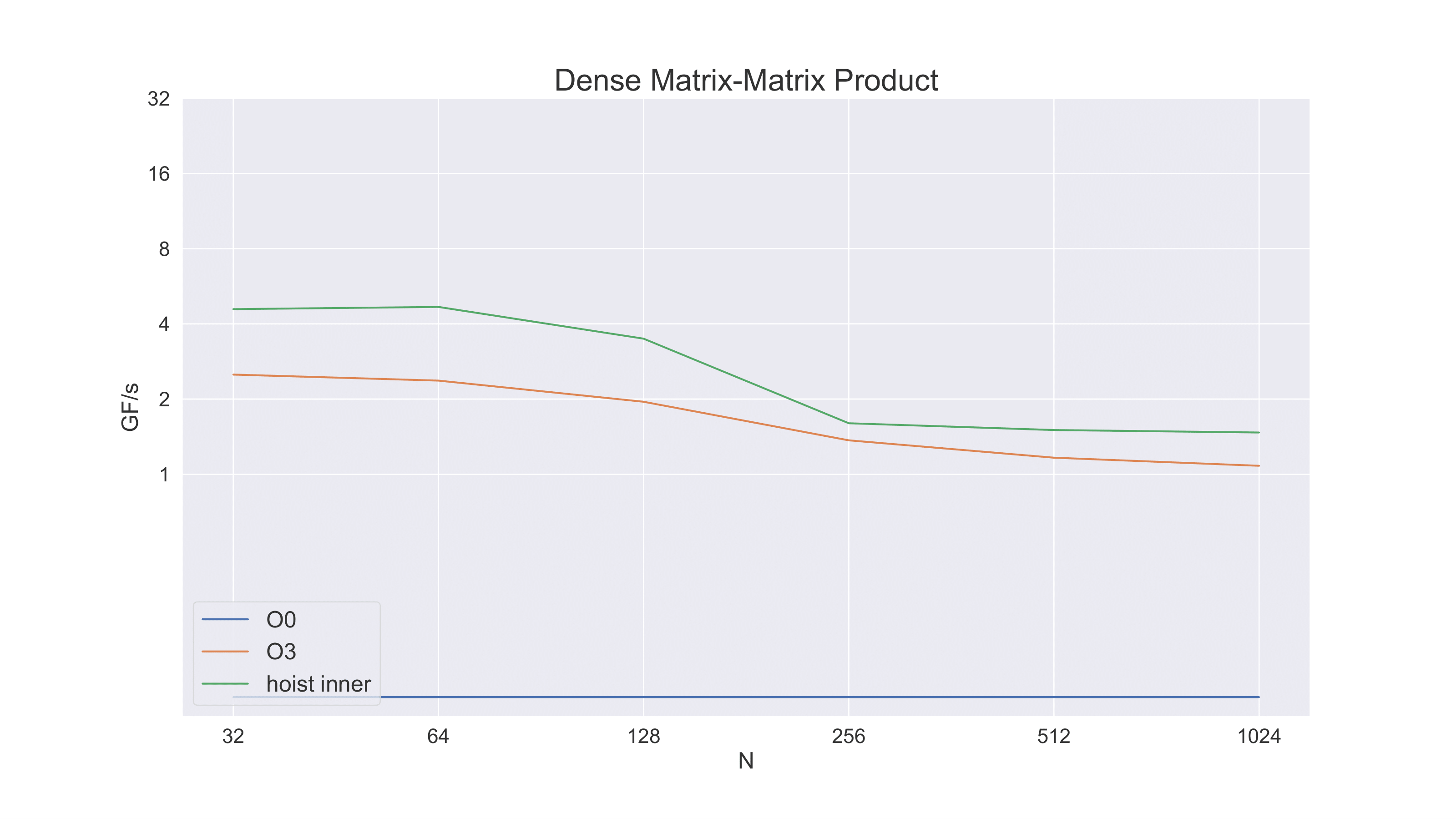
Note what this does immediately to efficiency. Now there are only four operations in the inner loop: two memory accesses and two floating point operations. Our efficiency has gone from 1/3 to 1/2 simply by moving C(i,j) out of the inner loop.

And, in fact, performance improves significantly with just this simple technique.

Now we can also increase the reuse of A(i,k) and B(k,j) in the inner loop by unrolling their access, that is, by doing a two-by-two block multiply in the inner loop:

void multiply(const Matrix& A, const Matrix&B, Matrix&C) {
  for (size_t i = 0; i < A.num_rows(); i += 2) {
    for (size_t j = 0; j < B.num_cols(); j += 2) {
      for (size_t k = 0; k < A.num_cols(); ++k) {
        C(i  , j  ) += A(i  , k) * B(k, j  );
        C(i  , j+1) += A(i  , k) * B(k, j+1);
        C(i+1, j  ) += A(i+1, k) * B(k, j  );
        C(i+1, j+1) += A(i+1, k) * B(k, j+1);
      }
    }
  }
}

We can combine this with hoisting, but now we need to hoist the two-by-two block of C out of the inner loop.

void multiply(const Matrix& A, const Matrix&B, Matrix&C) {
  for (size_t i = 0; i < A.num_rows(); i += 2) {
    for (size_t j = 0; j < B.num_cols(); j += 2) {
      double t00 = C(i,  j);     double t01 = C(i,  j+1);
      double t10 = C(i+1,j);     double t11 = C(i+1,j+1);
      for (size_t k = 0; k < A.num_cols(); ++k) {
        t00 += A(i  , k) * B(k, j  );
        t01 += A(i  , k) * B(k, j+1);
        t10 += A(i+1, k) * B(k, j  );
        t11 += A(i+1, k) * B(k, j+1);
      }
      C(i,  j) = t00;  C(i,  j+1) = t01;
      C(i+1,j) = t10;  C(i+1,j+1) = t11;
    }
  }
}

Now let’s count operations in the inner loop. There are four total memory accesses for A and B but now there are eight floating point operations – an efficiency of 2/3 – twice what we started with. The next plot shows the performance benefit (we also show the result of unrolling without hoisting). Note that although performance improves greatly for the small problem sizes, it still falls off for larger problem sizes.

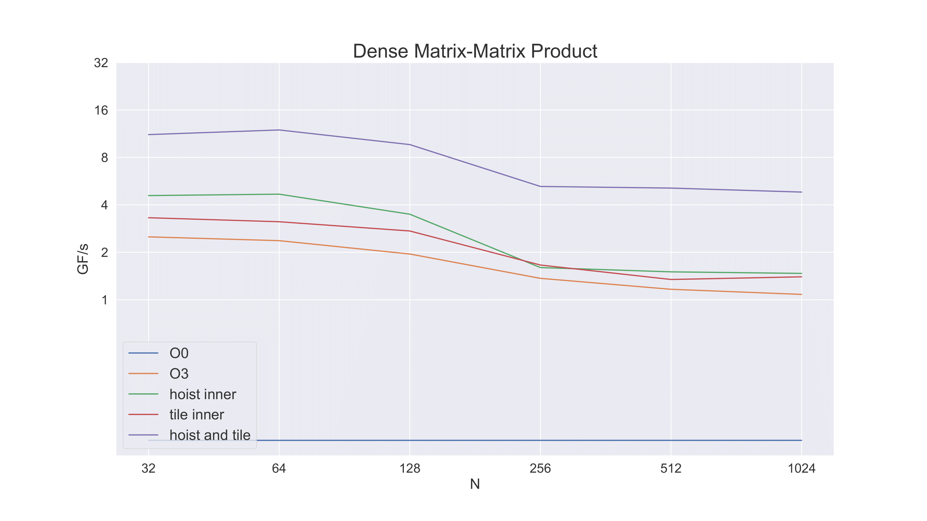
Next we note that matrix-matrix product for a large matrix can be decomposed into blocks of matrix-matrix products with small matrices. If we perform our operations this way, we should be able to maintain a higher level of performance for larger problems.

Finally, we note that we can get better cache behavior yet – and a more favorable access pattern, if B is in the transpose orientation of A. For memory efficiency reasons we don’t make a transpose copy of all of B for the multiplication. Rather we only need to make a transpose copy of the block of B that we are working on in the blocked version of the algorithm.

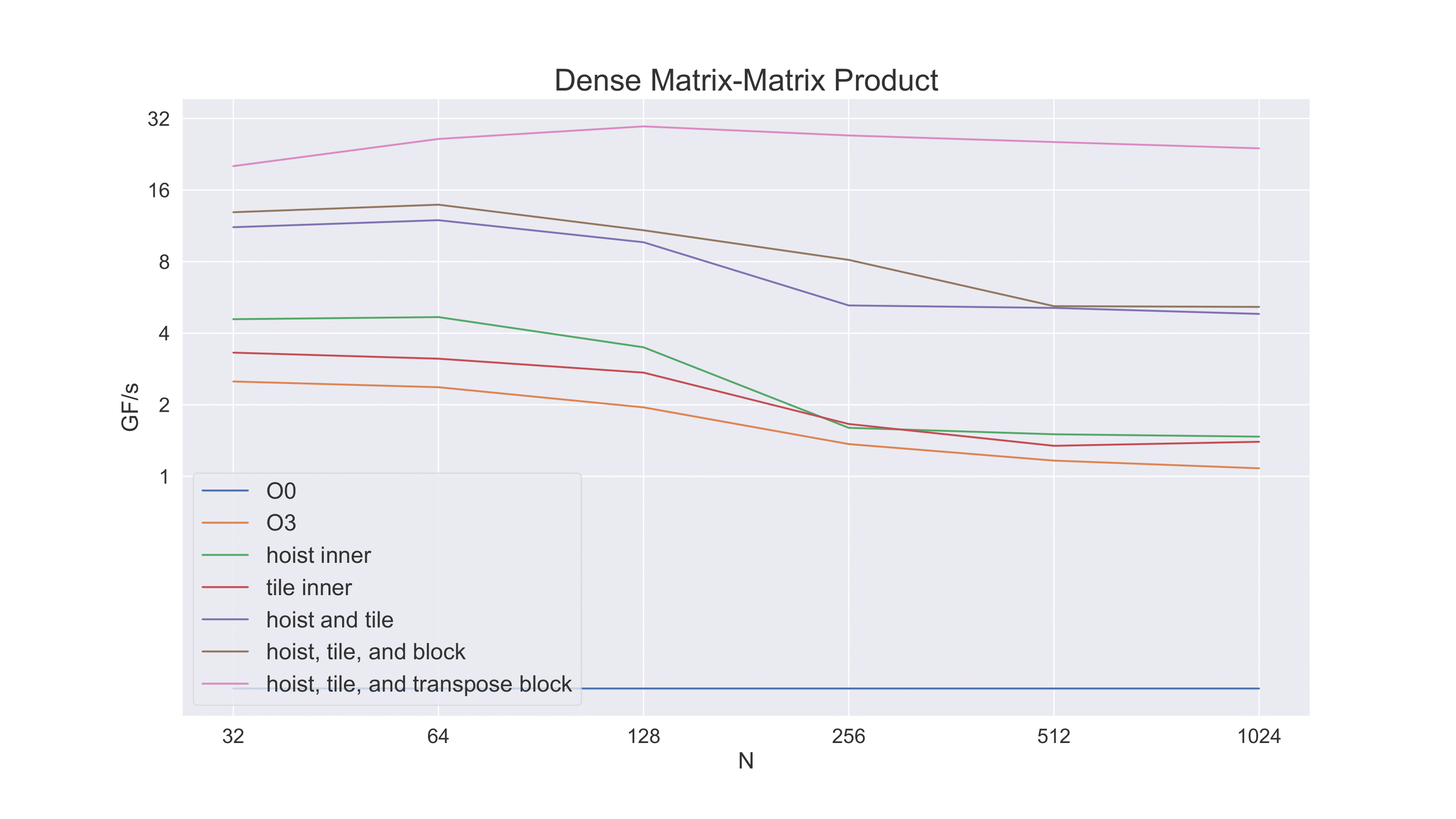
Notice how much performance has improved from our first, naive, implementation of the algorithm. We’ve gone from one or two GFlop/s to over 32.

Vector Instructions¶

But wait. In our model of CPU computation we considered one operation per clock cycle to be the most that could be done. In the best case above, we are getting 32 GFlop/s – but the laptop that the operation ran on only has a 2.4GHz clock. If the computer had no memory accesses at all and only did floating point operations, we would expect a peak performance rate of 2.4GFlop/s. With memory accesses taken into account, we could get 2/3 efficiency, or about 1.6 GFlop/s.

How are we getting 32 GFlop/s – twenty times what is predicted?

Twenty times the predicted performance rate means we are essentially doing 20 floating point operations where we thought we could only do one.

The first source of multiple operations per clock cycle comes from a special operation: fused multiply-add. That is, modern microprocessors (that have fused multiply add) can do the inner multiply and add for matrix-matrix product in a single clock cycle. That still leaves a factor of ten that needs to be accounted for.

A second source of improvement comes from clock rate. Although the microprocessor in the target laptop is spec’d at 2.4GHz, it is able to burst computations at a higher clock rate, up to a factor of two higher in fact (though this cannot be sustained). Let’s say that accounts for another 20% – that still leaves a factor of eight.

This factor of eight is achieved through the use of vector instructions. That is, rather than performing an operation (in this case, fused multiply-add) on two operands at a time, the microprocessor can perform the operation on multiple operands at a time. The target CPU for these experiments includes AVX512 instructions – instructions that can operate on data 512 bits wide. Since a double precision floating point number is eight bytes (or 64 bits), eight floating point values can fit into an AVX512 register – thereby accounting for our final factor of eight in performance.