Lecture 9: Strassen’s Algorithm. Sparse Matrices.


(Recorded on 2022-04-26)
So far we have been looking at how to extract maximum performance (in terms of floating point operations per second) from a CPU. However, in the larger context of scientific computing and problem solving, ultimately what we want to do is compute the answer the in the shortest amount of time.
In this lecture we look at a couple of ways to work smarter (and to work less) in order to reduce time to solution.
We first look at a remarkable algorithm discovered by Volker Strassen (and which now bears his name): Strassen’s algorithm for computing matrix-matrix product with lower than \(N^3\) computational complexity.
Next we develop a representation for matrix storage that stores only the information we need for representing a problem and that also results in significant improvements in time to solution.
Sparse Matrix Computations
“High-Performance Scientific Computing” covers a large (and growing) intellectual space. A core theme in scientific computing is using computer algorithms (which are necessarily discrete, at least in digital computers) to model physical phenomena (which are necessarily continuous). The physical phenomena are also typically modeled mathematically as systems of nonlinear partial differential equations, which require discretization and linearization to reduce them (within the context of a larger iterative solution process) to systems of linear equations, aka \(\mat{A}\vec{x}=\vec{b}\).
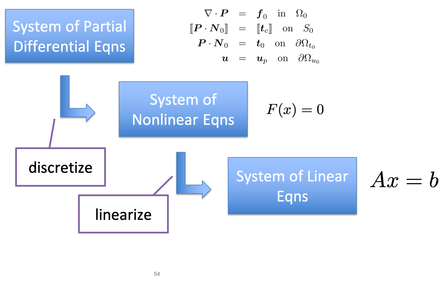
The matrices at the bottom of this sequence of steps have an important characteristic: Almost all of the entries are zero. Computations using such a matrix thus involve adding and multiplying zero elements, operations which essentially have no effect and could be profitably eliminated. To do so, we need to develop special data structures—sparse matrix data structures—that only store the non-zero entries of the matrix, but allow us to perform operations such as matrix-vector product.
Example: Laplace’s Equation
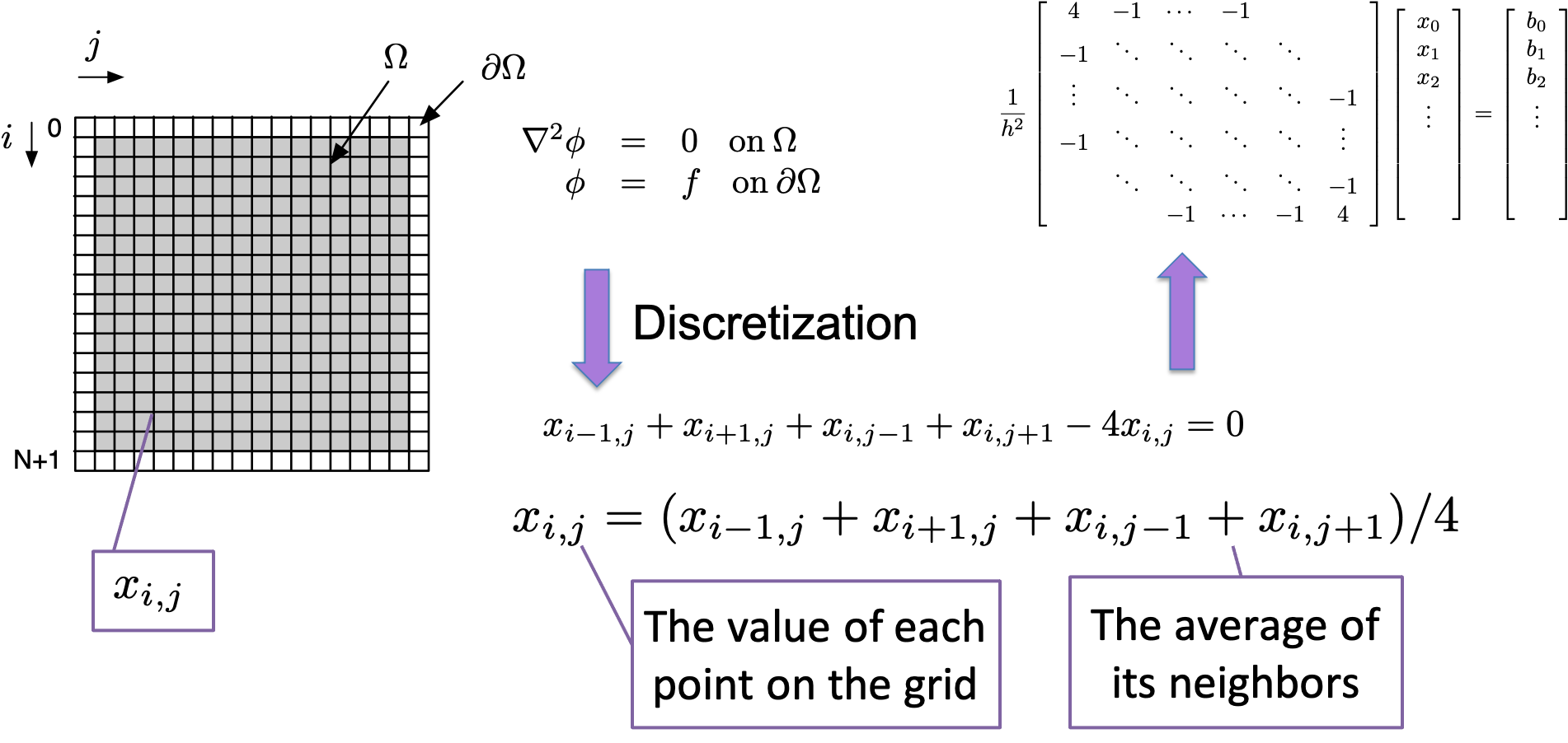
Laplace’s equation on a unit square is a prototypical PDE that we can use to derive sparse matrix data structures
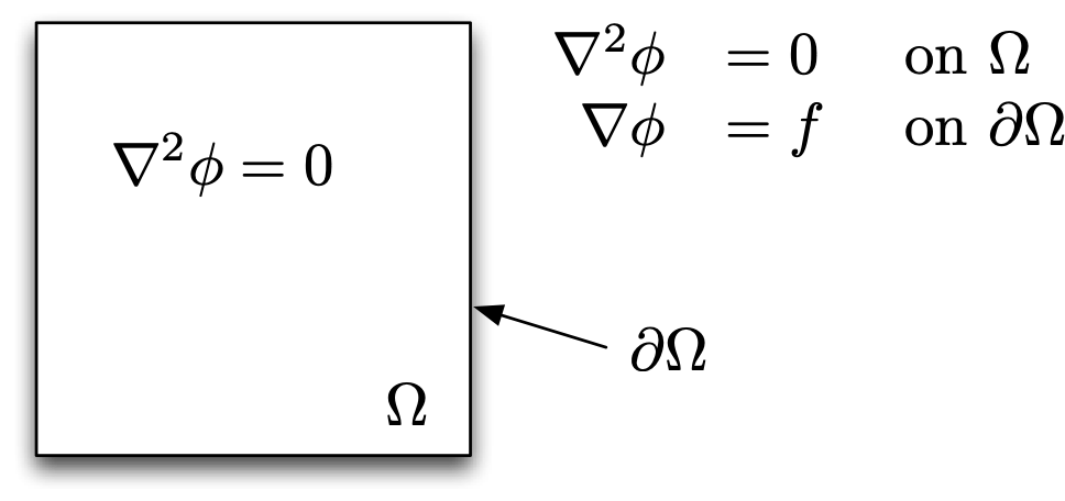
If we discretize the domain, we turn our continuous differential equation into an algebraic equation by using a finite-difference approximation to the differential operator.
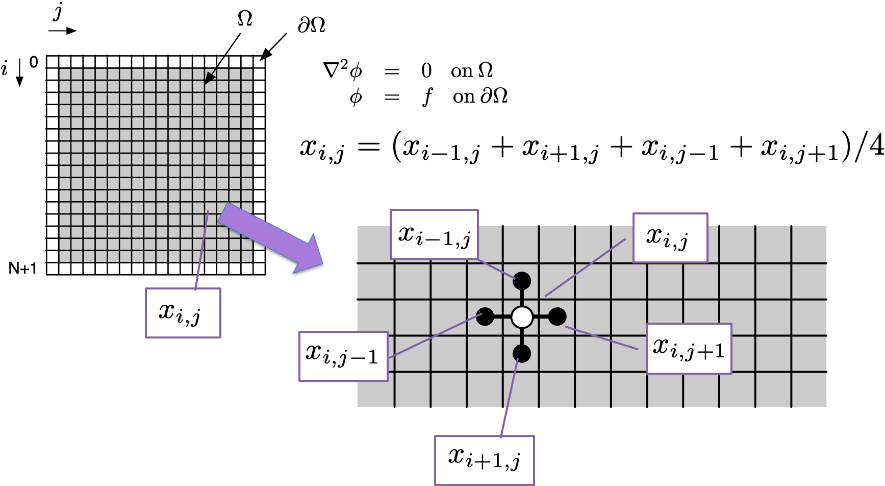
We can collect the equations for each grid point in the discretized domain into a collection of simultaneous equations, i.e., a linear system of equations. The coefficients and variables can be represented in matrix form \(\mat{A}\vec{x}=\vec{b}\).
Important
Make sure you can explain how we go from the stencil to \(\mat{A}\vec{x}=\vec{b}\) (cf slides 24 and 25).
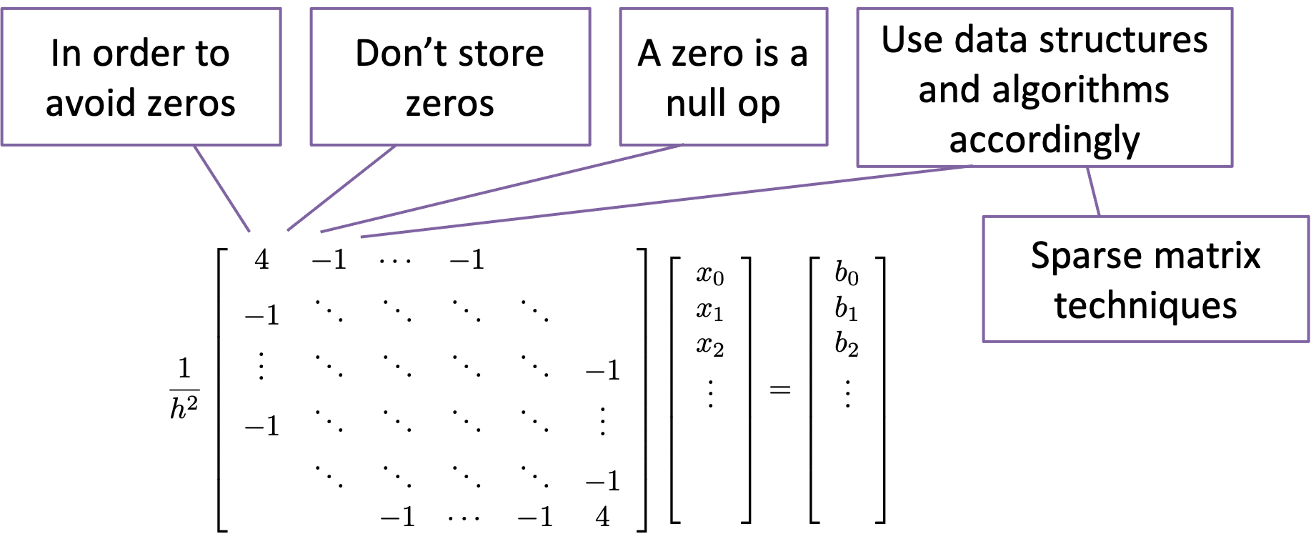
Each of the equations that comprise the matrix system have only five coefficients, meaning that there are only five non-zero elements on each row of the matrix—regardless of the matrix size. For a domain that is discretized with 1,000 points in each dimension, the matrix size will be 1M by 1M — but with only five elements per row. Clearly, a representation that stores only the non-zero elements (of which there are 5,000) is much more efficient than one that stores all of the elements (of which there are 1M). Sparse matrix techniques include both the data structures as well as the algorithms that are used to exploit the non-zero structure.
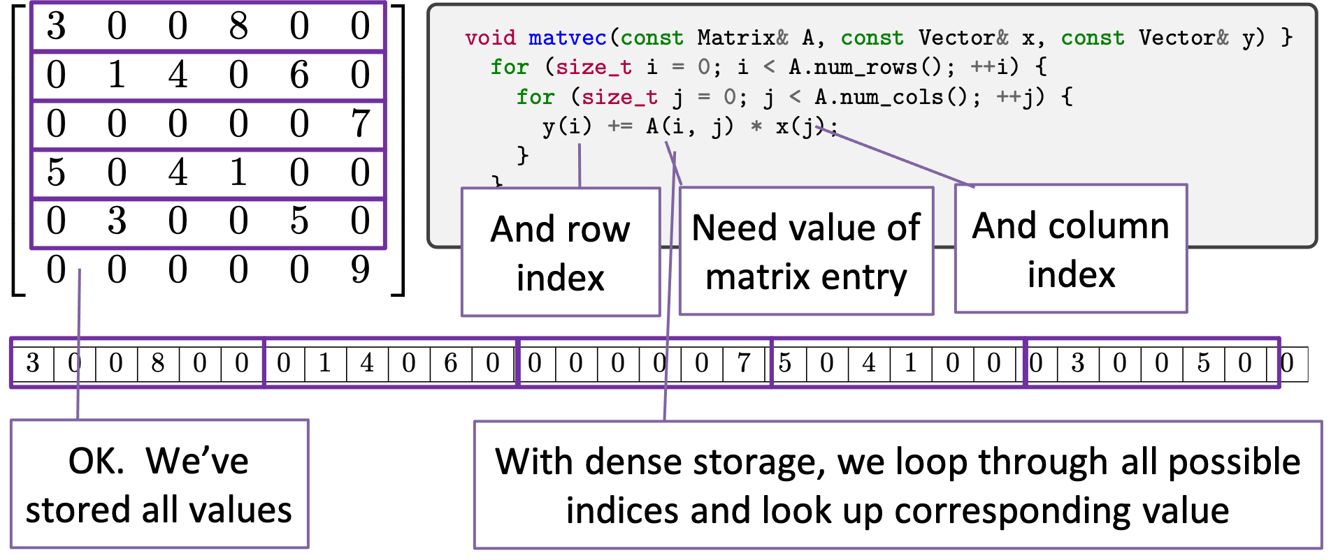
To do a computation such as matrix-vector product (which is the canonical sparse matrix operation) we need the row, column, and data value of the matrix entry. In the case of dense matrix-vector product, the row and column are obtained by our loop variables as we iterate through the rows and columns of the matrix.
For a sparse matrix, we no longer store all of the matrix entries, but only some of them. In the sparse matrix-vector product, we iterate just over the non-zero entries in the matrix. But for the algorithm we still need the row index and column index corresponding to the non-zero matrix entry. Since we can’t implicitly infer the row and column indices from the location of the entry in the matrix (from our loop indices), we need to instead explicitly store them.
Coordinate Storage
The most basic sparse matrix storage format is coordinate storage, which, for each matrix non-zero entry, stores the entry’s value, row index, and column index.
One possible implementation for coordinate storage as a C++ class might look like:
class COOMatrix {

public:
  COOMatrix(size_t M, size_t N) : num_rows_(M), num_cols_(N) {}

  size_t num_rows() const { return num_rows_; }
  size_t num_cols() const { return num_cols_; }

private:
  size_t              num_rows_, num_cols_;
  std::vector<size_t> row_indices_, col_indices_;
  std::vector<double> storage_;
};
In this storage format we use std::vector to store the value, row index, and
column index information. These vectors will all be the same size. For a given index
value k, which will be less than the size of the vectors, the quantities
storage[k], row_indices[k], and col_indices[k] represent the
corresponding value, row index, and column index for the kth non-zero in the matrix.
There is a crucial thing to notice about this format (and which is a consequence of
only storing non-zero entries): there is no random access to elements, that is, there
is no operator() to access entries by their row and column number. With dense
matrices, we used operator() to access the internal data of the matrix.
Without operator() That means we need a different approach for expressing
algorithms. In particular, we will need to implement algorithms such as matrix-vector
product as member functions of the sparse matrix structure.
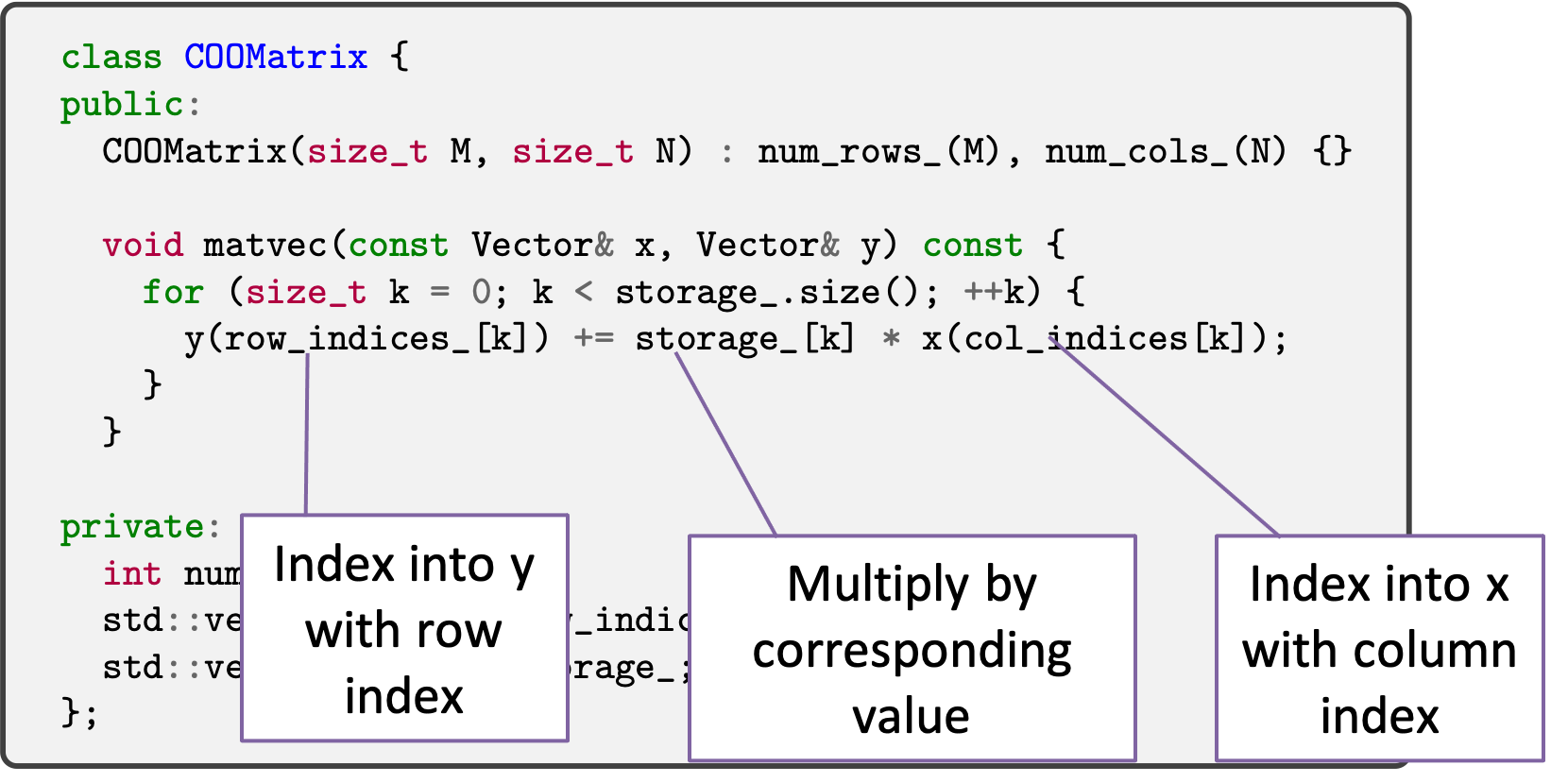
To develop a matrix-vector product for coordinate format, consider dense matrix-vector product:
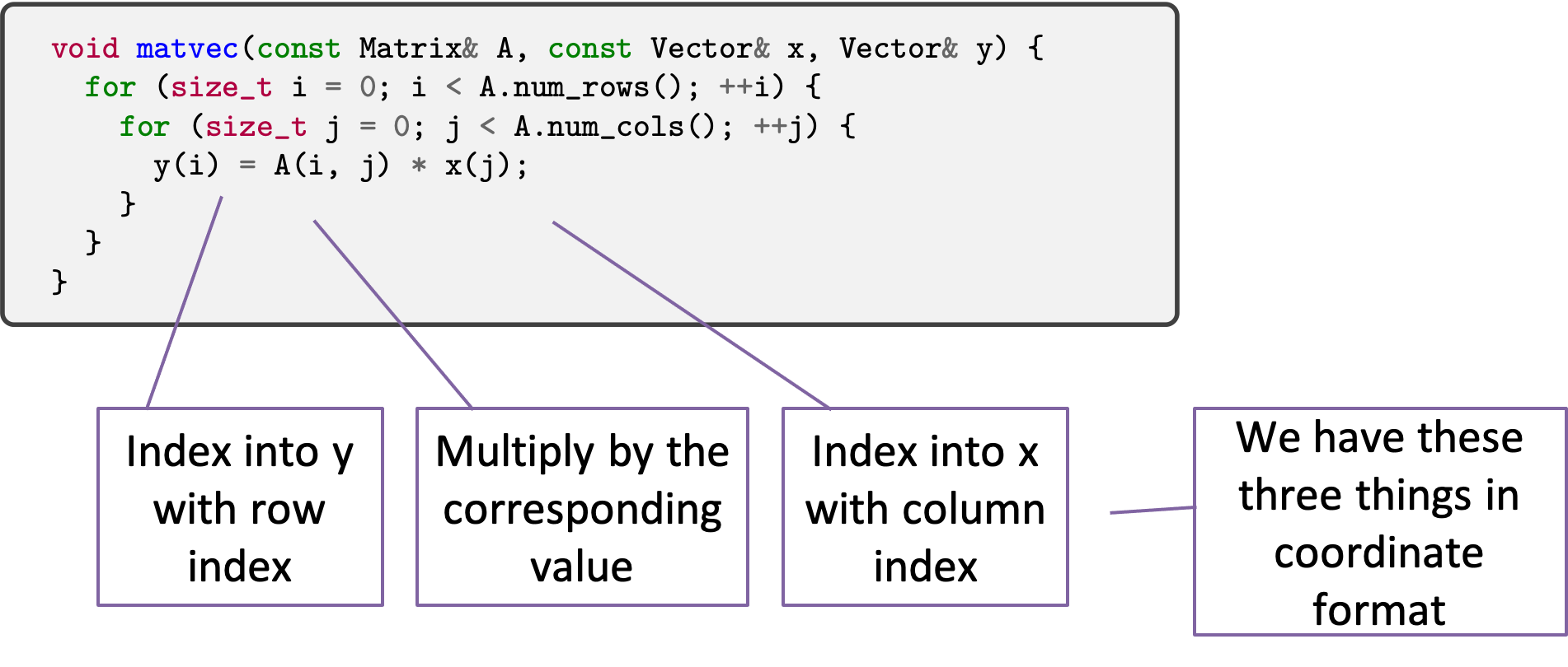
Consider what we are doing abstractly. We are going through every element in the
matrix. At each element, we index into y with the row index and index into
x with the column index and we multiply the entry’s value against the retrieved
value of x and store that product into y.
We can do exactly this abstract operation for our coordinate storage.
That is, we can go through every element in the matrix, we can index into y
with the row index, we can index into x with the column index, and we can
obtain the matrix value to do multiply against. This is expressed differently for the
coordinate storage format
Important
Make sure you can explain how coordinate matrix-vector product and dense matrix-vector product are performing the same abstract operation.
We note that the numerical intensity of sparse matrix-vector product is quite a bit lower than for dense matrices (cf slide 52). Nonetheless, sparse matrix computation can provide enormous performance benefits. See the excursus on Sparse vs Dense Computation (Or, How to be Faster while Being Slower).
Compressed Sparse Storage
The coordinate format is a basic and easy to use format. However, there are some ways to make sparse storage more compact and more efficient. We achieve this by compressing one of the index axes (either the rows or the columns) and thereby reduce some redundancy and improve locality. Our steps for compression will be to first sort the matrix entries according to one of the index axes, then run-length encode the resulting array, then perform a prefix sum along the run-length encoded array.
The example we will look at will be sorting and compressing along the row index array and will result in the compressed sparse row (CSR) format. A similar process can be followed for compressing along the column index array to arrive at the compressed sparse column (CSC) format. CSR is probably the most common sparse matrix format used in scientific computing today.
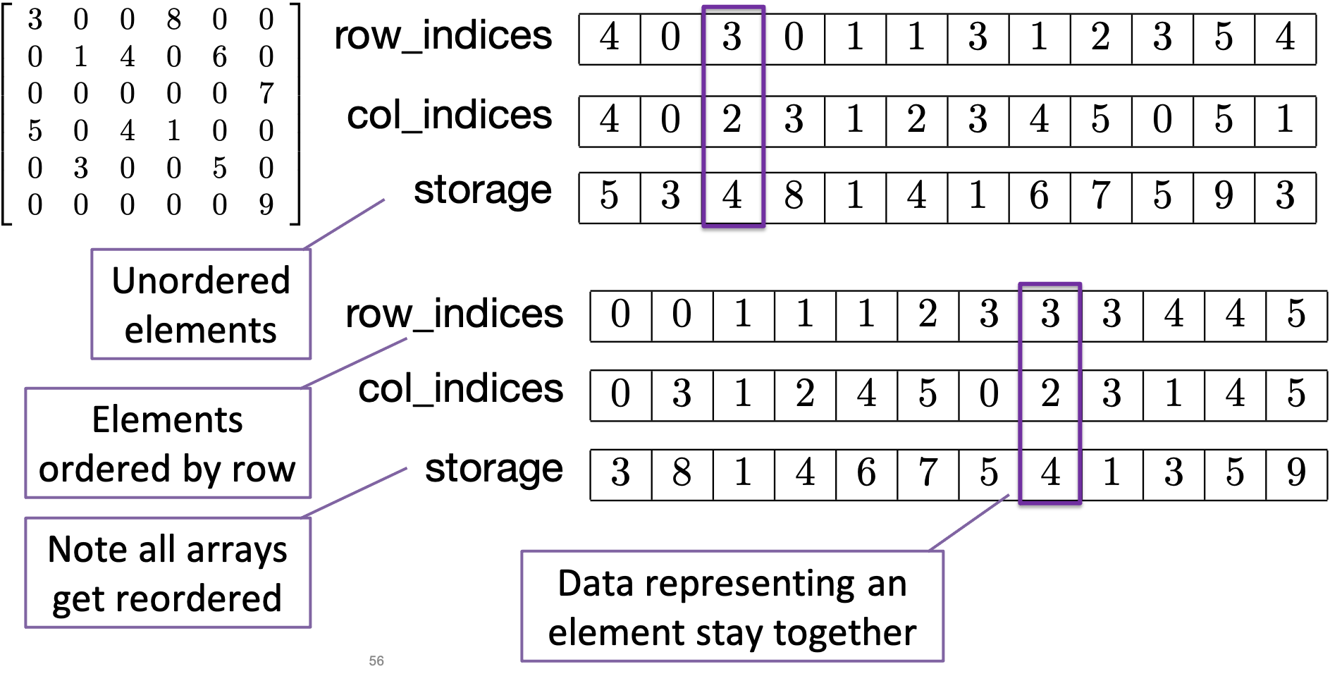
Next, we note that there are repeated entries for each row value. We can reduce the size of this array by applying
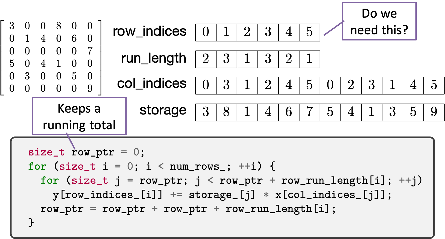
The data necessary to represent a matrix in Compressed Sparse Row (CSR) format are thus

An implementation of CSR as a C++ class might look like:
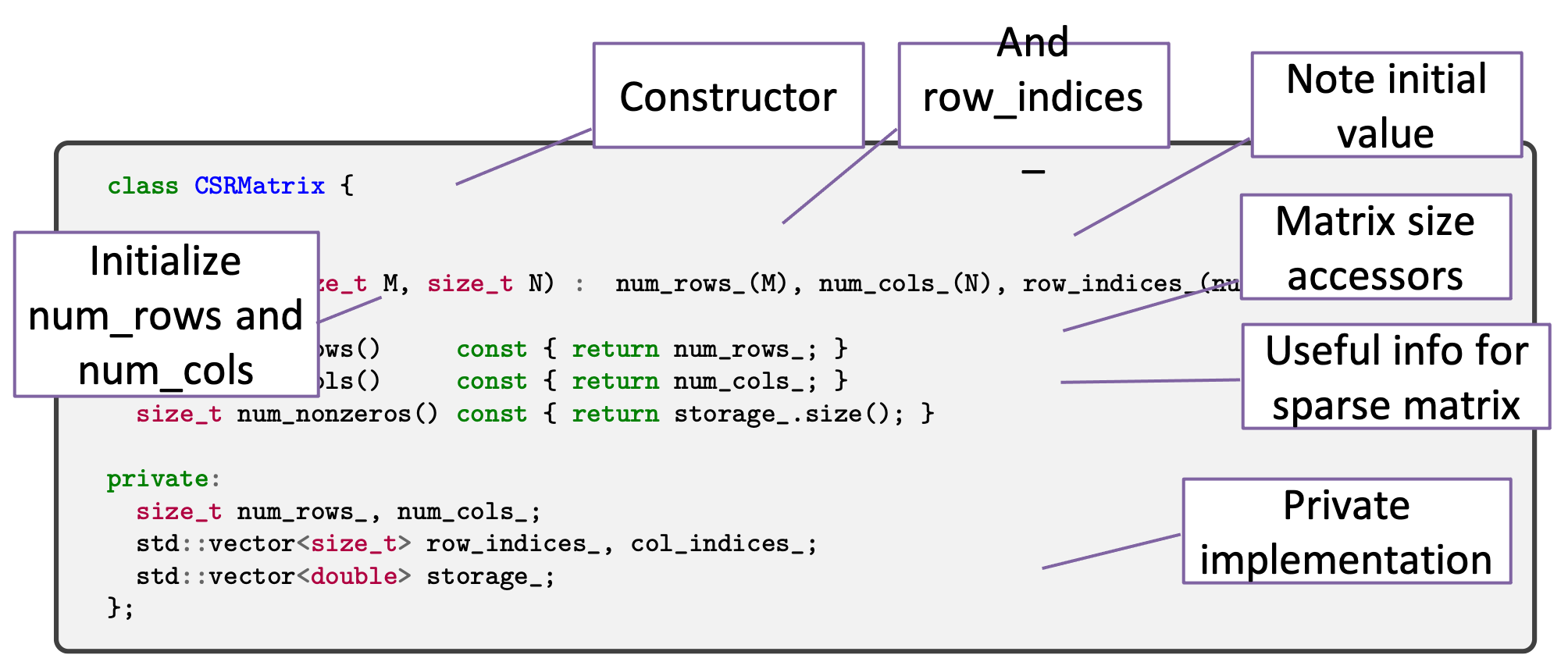
An implementation of matrix-vector product for CSR might look like.
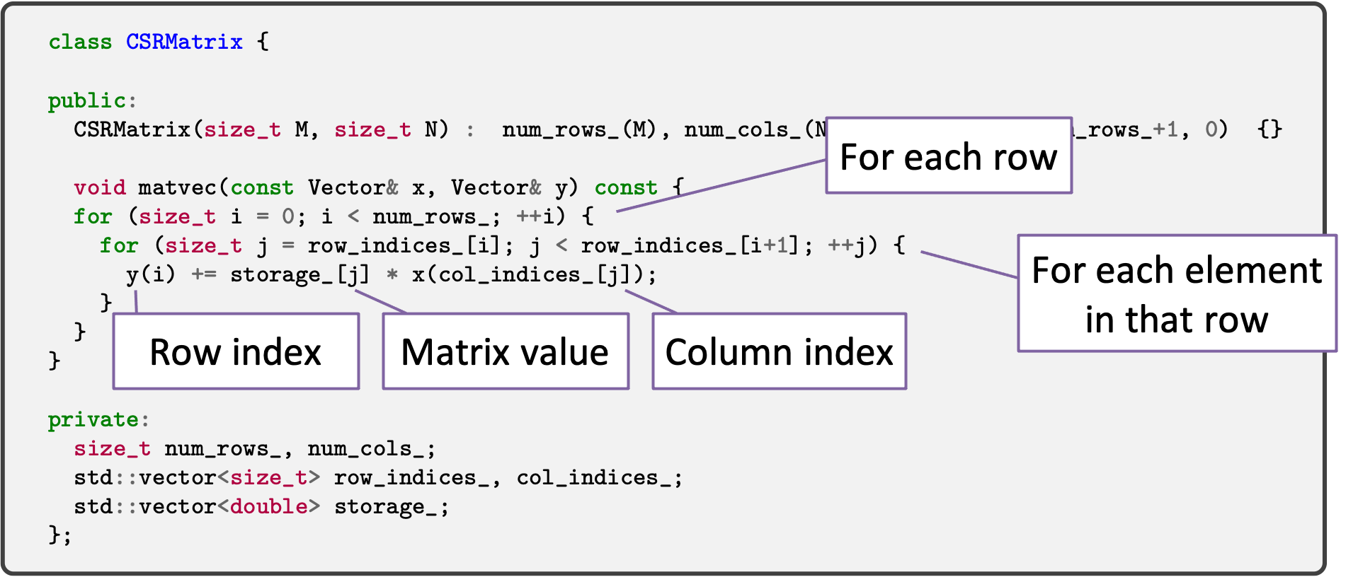
Again, the matrix-vector product follows the abstract matrix-vector operation that we
presented above. However, due to the way we are storing matrix entries, we use a
two-level loop structure. That is, we iterate through the rows and then iterate over
the elements in that row. (Another way to think about CSR is that we have put all of
the elements in every row together and that neighboring values in the
row_indices_ array point to the beginning and and of the elements in that row,
as stored in the col_indices_ and storage_ arrays.)
Important
Make sure you can explain how to derive CSR from COO.
Important
Make sure you can explain how CSR is performing the abstract matrix-vector product operation.