Problem Set #5¶

Extract the homework files¶

Create a new subdirectory named “ps5” to hold your files for this assignment. The files for this assignment are in a “tar ball” that can be downloaded with ps5.tar.gz.

To extract the files for this assignment, download the tar ball and copy it (or move it) to your ps5 subdirectory. From a shell program, change your working directory to be the ps5 subdirectory and execute the command

$ tar zxvf ps5.tar.gz

The files that should be extracted from the tape archive file are

• AOSMatrix.hpp: Header file for array-of-structs sparse matrix

• COOMatrix.hpp: Header file for coordinate struct-of-arrays sparse matrix

• CSCMatrix.hpp: Header file for compressed sparse column matrix

• CSRMatrix.hpp: Header file for compressed sparse row matrix

• Makefile: Makefile

• Matrix.hpp: Header for simple dense matrix class

• Timer.hpp: Header for simple timer class

• Vector.hpp: Header for simple vector class

• amath583.{cpp,hpp}: Source and header for basic math operations

• amath583IO.{cpp,hpp}: Source and header for file I/O

• amath583sparse.{cpp,hpp}: Source and header for sparse operations

• bonnie_and_clyde.cpp, bonnie_and_clyde_function_object.cpp: Demo files for bonnie and clyde

• catch.hpp: Catch2 header file

• cnorm.{cpp,hpp}, cnorm_test.cpp: Driver, header, and test program for cyclic parallel norm

• data/ : Some test data files (including Erdos02)

• fnorm.{cpp,hpp}, fnorm_test.cpp: Driver, header, and test program for task based parallel norm

• matvec.cpp, matvec_test.cpp: Driver and test programs for sparse matrix-vector product

• norm_order.cpp, norm_test.cpp: Driver test and program for different implementations of two_norm

• norm_utils.hpp: Helper functions for norm driver programs

• pagerank.{cpp,hpp}, pagerank_test.cpp: Driver, header, and test program for pagerank

• pmatvec.cpp, pmatvec_test.cpp: Parallel matvec driver and test programs

• pnorm.{cpp,hpp}, pnorm_test.cpp: Driver, header, and test program for block partitioned parallel norm with threads

• pr.py: Python pagerank implementation

• rnorm.{cpp,hpp}, rnorm_test.cpp: Driver, header, and test program for divide-and-conquer parallel norm

• verify-{all,make,opts,run,test}.bash: Verification scripts for programs in this assignment

You may or may not notice, in this makefile of this assignment, we have updated from C++11 to C++17 for the C++ language standard. Many new features have been added to C++17 comparing with C++11, or C++14.

std::Futures¶

C++ provides the mechanism to enable execution of a function call as an asynchronous task. Its semantics are important. Consider the example we have been using in lecture.

typedef size_t size_t;

size_t bank_balance = 300;

static std::mutex atm_mutex;
static std::mutex msg_mutex;

size_t withdraw(const std::string& msg, size_t amount) {
  std::lock(atm_mutex, msg_mutex);
  std::lock_guard<std::mutex> message_lock(msg_mutex, std::adopt_lock);

  std::cout << msg << " withdraws " << std::to_string(amount) << std::endl;

  std::lock_guard<std::mutex> account_lock(atm_mutex, std::adopt_lock);

  bank_balance -= amount;
  return bank_balance;
}

int main() {
  std::cout << "Starting balance is " << bank_balance << std::endl;

  std::future<size_t> bonnie = std::async(withdraw, "Bonnie", 100);
  std::future<size_t> clyde  = std::async(deposit, "Clyde", 100);

  std::cout << "Balance after Clyde's deposit is " << clyde.get() << std::endl;
  std::cout << "Balance after Bonnie's withdrawal is " << bonnie.get() << std::endl;

  std::cout << "Final bank balance is " << bank_balance << std::endl;

  return 0;
}

Here we just show the withdraw function. Refer to the full source code for complete implementation bonnie_and_clyde.cpp .

Note that we have modified the code from lecture so that the deposit and withdrawal functions return a value, rather than just modifying the global state.

Compile and run the bonnie_and_clyde program several times. Does it always return the same answer?

On my laptop I ran the example and obtained the following results (which were different every time):

$ ./bonnie_and_clyde.exe
Starting balance is 300
Bonnie withdraws 100
Balance after Clyde\'s deposit is Clyde deposits 100
300
Balance after Bonnie\'s withdrawal is 200
Final bank balance is 300

$ ./bonnie_and_clyde.exe
Starting balance is 300
Balance after Clyde\'s deposit is Clyde deposits 100
Bonnie withdraws 100
400
Balance after Bonnie\'s withdrawal is 300
Final bank balance is 300

$ ./bonnie_and_clyde.exe
Starting balance is 300
Bonnie withdraws 100
Clyde deposits 100
Balance after Clyde\'s deposit is 300
Balance after Bonnie\'s withdrawal is 200
Final bank balance is 300

$ ./bonnie_and_clyde.exe
Starting balance is 300
Balance after Clyde\'s deposit is Bonnie withdraws 100
Clyde deposits 100
300
Balance after Bonnie\'s withdrawal is 200
Final bank balance is 300

See if you can trace out how the different tasks are running and being interleaved. Notice that everything is protected from races – we get the correct answer at the end every time.

Note the ordering of calls in the program:

std::future<size_t> bonnie = std::async(withdraw, "Bonnie", 100);
std::future<size_t> clyde  = std::async(deposit, "Clyde", 100);

std::cout << "Balance after Clyde's deposit is " << clyde.get() << std::endl;
std::cout << "Balance after Bonnie's withdrawal is " << bonnie.get() << std::endl;

That is, the ordering of the calls is Bonnie makes a withdrawal, Clyde makes a deposit, we get the value back from Clyde’s deposit and then get the value back from Bonnie’s withdrawal. In run 0 above, that is how things are printed out: Bonnie makes a withdrawal, Clyde makes a deposit, we get the value after Clyde’s deposit, which is 300, and we get the value after Bonnie’s withdrawal, which is 200. Even though we are querying the future values with Clyde first and Bonnie second, the values that are returned depend on the order of the original task execution, not the order of the queries.

But let’s look at run 2. In this program, there are three threads: the main thread (which launches the tasks), the thread for the bonnie task and the thread for the clyde task. The first thing that is printed out after the tasks are launched is from Clyde’s deposit. But, before that statement can finish printing in its entirety, the main thread interrupts and starts printing the balance after Clyde’s deposit. The depositing function isn’t finished yet, but the get() has already been called on its future. That thread cannot continue until the clyde task completes and returns its value. The clyde task finishes its cout statement with “100”. But then the bonnie task starts running - and it runs to completion, printing “Bonnie withdraws 100” and it is done. But, the main thread was still waiting for its value to come back from the clyde task – and it does – so the main thread completes the line “Balance after Clyde’s deposit is” and prints “400”. Then the next line prints (“Balance after Bonnie’s withdrawal”) and the program completes.

Try to work out the sequence of interleavings for run 1 and run 3. There is no race condition here – there isn’t ever the case that the two tasks are running in their critical sections at the same time. However, they can be interrupted and another thread can run its own code – it is only the critical section code itself that can only have one thread executing it at a time. Also note that the values returned by bonnie and clyde can vary, depending on which order they are executed, and those values are returned by the future, regardless of which order the futures are evaluated.

std::cout << "Balance after Clyde's deposit is " << clyde.get() << std::endl;
std::cout << "Balance after Bonnie's withdrawal is " << bonnie.get() << std::endl;
std::cout << "Double checking Clyde's deposit " << clyde.get() << std::endl;

Callables¶

We have looked at two ways of specifying concurrent work to be executed in parallel: threads and tasks. Both approaches take an argument that represents the work that we want to be done (along with additional arguments to be used by that first argument). One kind of thing that we can pass is a function.

void pi_helper(int begin, int end, double h) {
  for (int i = begin; i < end; ++i) {
    pi += (h*4.0) / (1.0 + (i*h*i*h));
  }
}

int main() {

  // ...

  std::thread(pi_helper, 0, N/4, h);  // pass function

  return 0;
}

The interfaces to thread and to async are quite general. In fact, the type of the thing being passed in is parameterized. What is important about it is not what type it is, but rather what kinds of expressions can be applied to it.

To be more concrete, the C++11 declaration for async is the following:

template< class Function, class... Args>
std::future<std::result_of_t<std::decay_t<Function>(std::decay_t<Args>...)>>
async( Function&& f, Args&&... args );

There are a number of advanced C++ features being used in this declaration, but the key thing to note is that, indeed, the first argument f is of a parameterized type (Function).

The requirements on whatever type is bound to Function are not that it be a function, but rather that it be Callable. Meaning, if f is Callable, we can say this as a valid expression:

f();

Or, more generally

f(args);

This is purely syntactic – the requirement is that we be able to write down the name of the thing that is Callable, and put some parentheses after it (in general with some other things inside the parentheses).

Of course, a function is one of the things that we can write down and put some parentheses after. But we have also seen in C++ that we can overload operator() within a class. Objects of a class with operator() can be written down with parentheses – just like a function call. In fact, this is what we have been doing to index into Vector and Matrix.

We can also create expressions that themselves are functions (“anonymous functions” or lambda expressions).

One way of thinking about thread and async is that they are “higher-order functions” – functions that operate on other functions. As you become more advanced in your use of C++, you will find that many common computational tasks can be expresses as higher order functions.

A bit more information about function objects and lambdas can be found as excursus: Function Objects and Lambda . Lambda is also covered in Lecture 13. There is also an example of function objects for our bank account example in the file bonnie_and_clyde_function_object.cpp.

Parallel Roofline¶

We have been using the roofline model to provide some insight (and some quantification) of the performance we can expect for sequential computation, taking into account the capabilities of the CPU’s compute unit as well as the limitations imposed by the memory hierarchy. These same capabilities and limitations apply once we move to multicore (to parallel computing in general). Some of the capabilities scale with parallelism – the available compute power scales with number of cores, as does the bandwidth for any caches that are directly connected to cores. The total problem size that will fit into cache also scales. Shared cache and main memory do not.

For the intrepid, you can run the docker images amath583/ert.openmp.2, amath583/ert.openmp.4, and amath583/ert.openmp to run the ERT on 2, 4, and 8 threads / cores. You can get the sequential profile from amath583/ert. Instructions are the same as from ps4.

Theoretically, the maximum performance of 8 cores should be 8 times than the maximum performance of single core, as well as the maximum bandwidth of L1/L2 caches (as they are private). The main memory bandwidth of 8 cores should stay the same as the main memory bandwidth of single core.

The sequential and 8 core results for my laptop are plotted as the following:

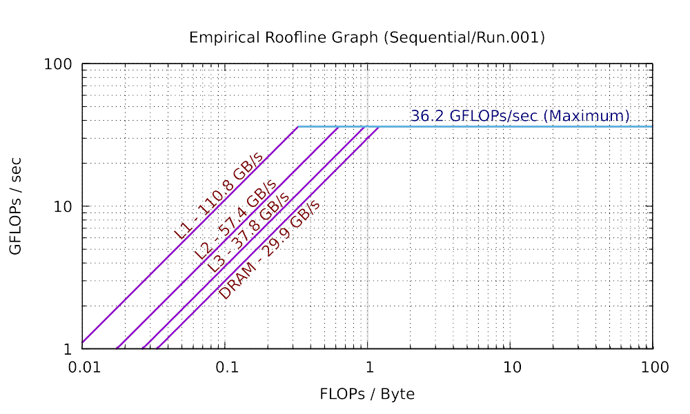
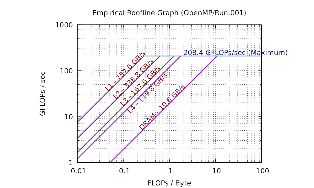
As you can see in practice, the maximum performance of 8 cores is 5.76 times (much smaller than 8 times) than the maximum performance of single core. The total bandwidth of the L1 cache of 8 cores is 6.84 times (still smaller than 8 times) than the bandwidth of the L1 cache of single core. You can observe similar trend in L2, and L3 caches. However, the bandwidth of the main memory of 8 cores is only has 66.2% of that of single core. This is because the main memory is shared among all cores. If you are not clear about why the parallel roofline model differs from the sequential roofline model, start a discussion on Piazza.

If you want to refer to a roofline model when analyzing some of your results for this assignment, you can either generate your own, refer to mine above, or estimate what yours would be based on what will and will not scale with number of cores.

Here are the sequential and parallel roofline results I got for Apple M1.

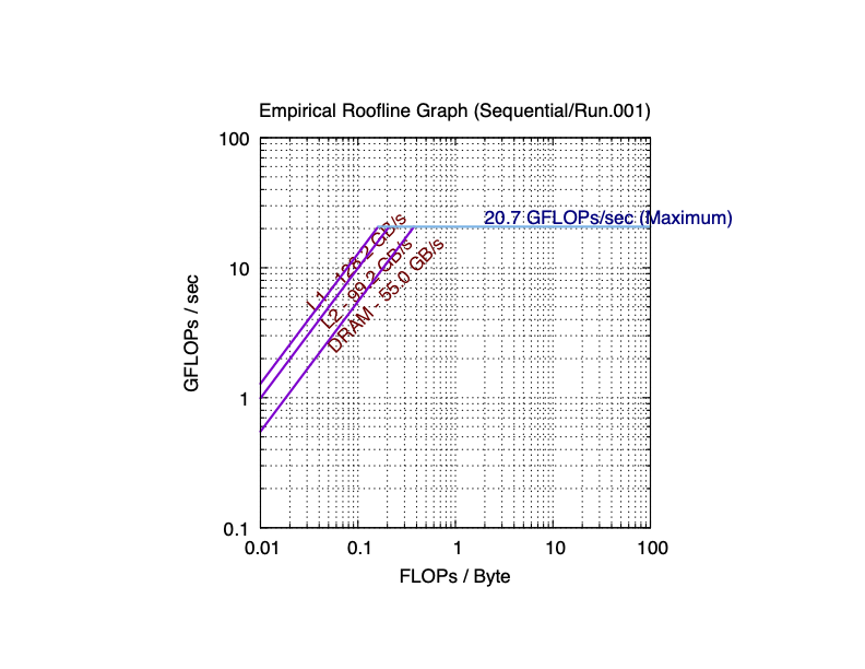
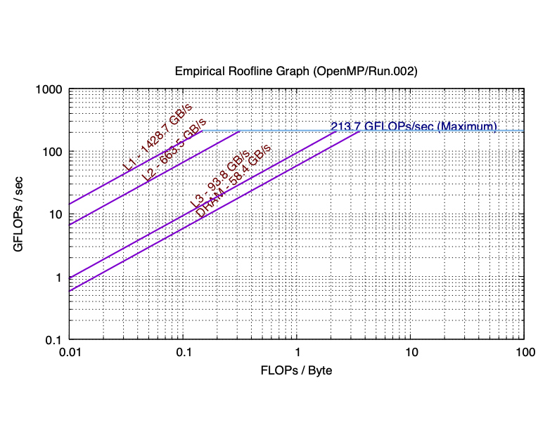
As you can see in practice, the maximum performance of 8 cores (according to Apple, M1 has 4 performance cores and 4 efficiency cores) is 10 times (more than 8 times) than the maximum performance of single core. The total bandwidth of the L1 cache of 8 cores is 11.1 times (still more than 8 times) than the bandwidth of the L1 cache of single core. For L2 cache, 8-core is 7.43 times than single core. L3 cache was failed to be detected on single core. However, the bandwidth of the main memory of 8 cores is very close to that of single core. This is because the main memory is shared among all cores. If you are not clear about why the parallel roofline model differs from the sequential roofline model, start a discussion on Piazza.

Here are the sequential and parallel roofline results I got for Apple M1 Max.

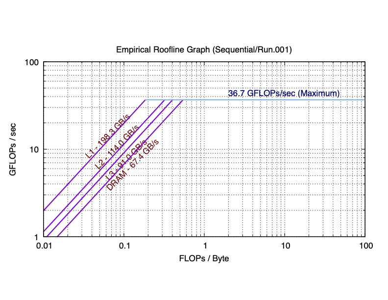
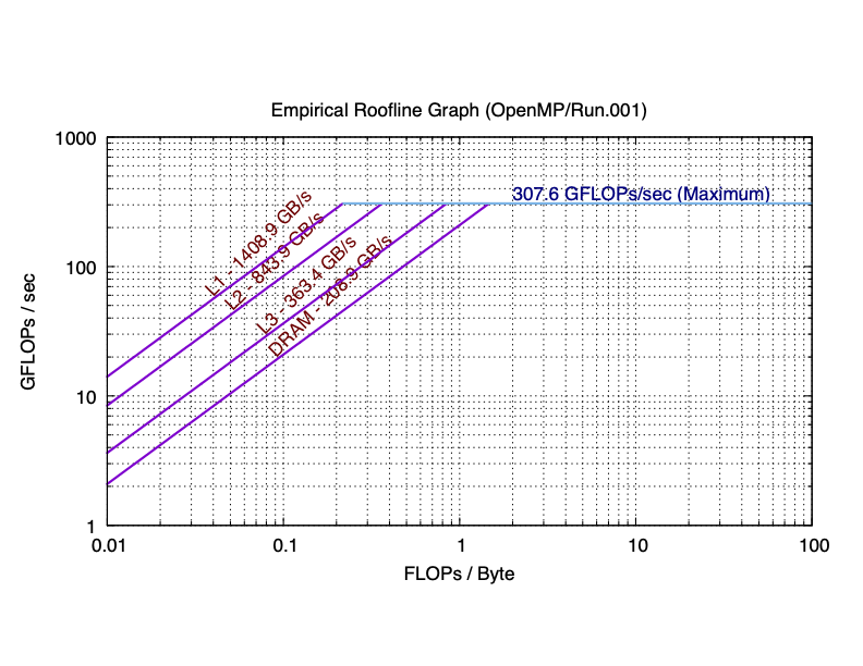
For M1 Max, I leave it for you to compute the performance difference in the plots.

Extra Credit¶

You may or may not notice that, since L1/L2 caches are private, the total bandwidth of them is definitively (much) more than that of the single core. However, because the DRAM is shared among all cores, the comparison between the bandwidth of the DRAM of 8 cores and that of the single core is more complicated. In the first Intel-CPU plot, we see the parallel bandwidth is smaller than the sequential one. In the Apple M1 plot, the parallel bandwidth is close to the sequential one. In the Apple M1 Max, the parallel bandwidth is almost 3 times than the sequential one.

If you are interested in this phenomenon, here is a hint for you to dive deep. What is the difference between SDRAM DDR4 and SDRAM DDR5 in terms of bandwidths? Wikipidia is a good starting point for investigation. DDR4 is the SDRAM type on my Intel machine and Apple M1 machine. Intel machine has one DRAM, Apple M1 machine has two. Hence the total bandwidths of Apple M1 will be twice than the bandwidth of the Intel machine. DDR5 is the DRAM type on Apple M1 Max machine, this machine has two of them (hence the total bandwidths will double). Why such difference would cause the bandwidth difference in the sequential roofline and the parallel roofline plots? You are welcomed to share your exploration process on Piazza.

Norm!¶

In lecture (and in previous assignments) we introduced the formal definition of vector spaces as a motivation for the interface and functionality of our Vector class. But besides the interface syntax, our Vector class needs to also support the semantics. One of the properties of a vector space is associativity of the addition operation, which we are going to verify experimentally in this assignment.

We have previously defined and used the function

double two_norm(const Vector&  x);

prototyped in amath583.hpp and defined in amath583.hpp.

In your source directory is a file norm_order.cpp that is the driver for this problem. It currently creates a Vector v and then invokes versions of two_norm on it four times, checking the results against that obtained by the first invocation.

The first invocation of two_norm is saved to the value norm0. We invoke two_norm a second time on v and save that value to norm1. We then check that norm0 and norm1 are equal.

As the program is delivered to you it also invokes two_norm_r on v and two_norm_s` on ``v (for “reverse” and “sorted”, respectively). The program also prints the absolute and relative differences between the values returned from two_norm_r and two_norm_s with the sequential two_norm to make sure the returned values are the same. The functions two_norm_r and two_norm_s are defined in amath583.cpp.

Absolute and relative differences are computed this way:

if (norm2 != norm0) {
  std::cout << "Absolute difference: " << std::abs(norm2-norm0) << std::endl;
  std::cout << "Relative difference: " << std::abs(norm2-norm0)/norm0 << std::endl;
}

(This is for norm2 - the code for the others should be obvious.)

Modify the code for two_norm_r in amath583.cpp so that it adds the values of v in reverse of the order given. I.e., rather than looping from 0 through num_rows()-1, loop from num_rows()-1 to 0.

for (size_t i = 0; i < x.num_rows(); ++i) {
   // ..
}

int main() {

  size_t i = 1;
  assert(i > 0);

  i = i - 1;       // subtract one from one
  assert(i == 0);

  i = i - 1;       // subtract one from zero
  assert(i < 0);

  return 0;
}

Modify the code for two_norm_s in amath583.cpp so that it adds the values of v in ascending order of its values. To do this, make a copy of v and sort those values using std::sort as follows

Vector w(v);  // w is a copy of v
std::sort(&w(0), &w(0)+w.num_rows());

What happens when you run norm_order.exe? Are the values of norm2 and norm3 equal to norm0?

Note that the program takes a command line argument to set the max size of the vector. The default is 1M elements.

Answer these questions in Questions.rst:

At what problem size (in terms of the number of elements in the Vector) do the answers between the computed norms start to differ?

How do the absolute and relative errors change as a function of problem size?

Does the Vector class behave strictly like an algebraic vector space?

Do you have any concerns about this kind of behavior?

Parallel Norm¶

For this problem we are going to explore parallelizing the computation of two_norm in a variety of different ways in order to give you some hands on experience with several of the common techniques for parallelization.

Each of the programs below consists of a header file for your implementation, a driver program, and a test program. The driver program runs the norm computation over a range of problem sizes, over a range of parallelizations. It also runs a sequential base case. It prints out GFlops/s for each problem size and for each number of threads. It also prints out the relative error between the parallel computed norm and the sequential computed norm.

Block Partitioning + Threads¶

Recall the approach to parallelization outlined in the Design Patterns for Parallel Programming. The first step is to find concurrency – how can we decompose the problem into independent (ish) pieces and then (second step) build an algorithm around that?

The first approach we want to look at with norm is to simply separate the problem into blocks. Computing the sum of squares of the first half (say) of a vector can be done independently of the second half. We can combine the results to get our final result.

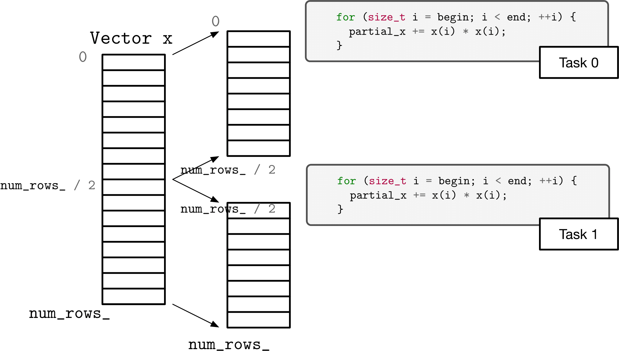
The program pnorm.cpp is a driver program that calls the function partitioned_two_norm_a in the file pnorm.hpp. The program as provided uses C++ threads to launch workers, each of which executes a specified block of the vector – from begin to end. Unfortunately, the program is not correct – more specifically, there is a race that causes it to give the wrong answer.

Fix the implementation of partitioned_two_norm_a in pnorm.hpp so that it no longer has a race and so that it achieves some parallel speedup. (Eliminating the race by replacing the parallel solution with a fully sequential solution is not the answer I am looking for.)

Answer the following questions in Questions.rst.

• What was the data race?

• What did you do to fix the data race? Explain why the race is actually eliminated (rather than, say, just made less likely).

• How much parallel speedup do you see for 1, 2, 4, and 8 threads?

Cyclic Partitioning + Your Choice¶

Another option for decomposing the two norm computation is to use a “cyclic” or “strided” decomposition. That is, rather than each task operating on contiguous chunks of the problem, each task operates on interleaved sections of the vector.

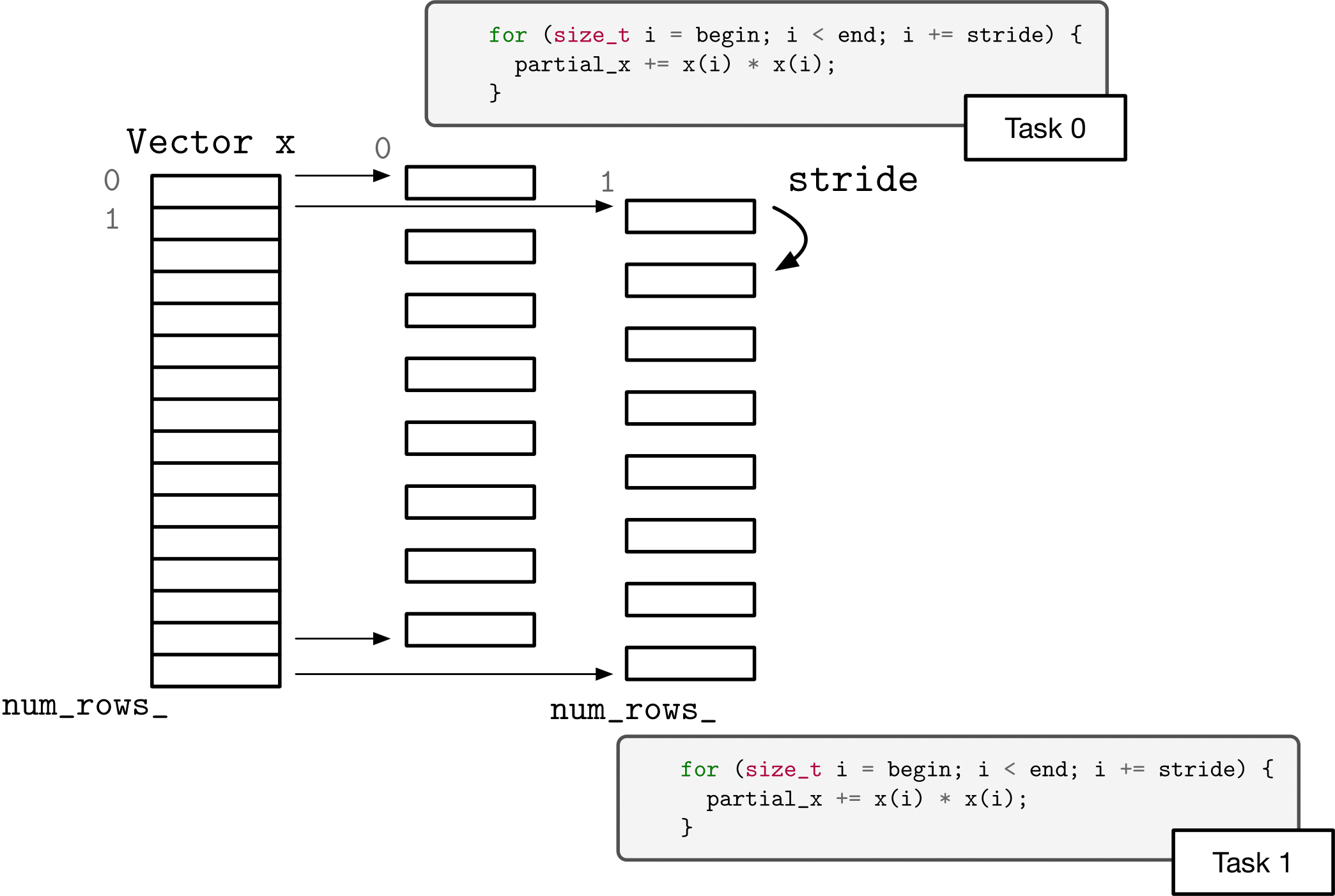
Complete the body of cyclic_two_norm in cnorm.hpp. The implementation mechanism you use is up to you (threads or tasks). You can use separate helper functions, lambdas, or function objects. The requirements are that the function parallelizes according to the specified number of threads, that it uses a cyclic partitioning (strides), and that it computes the correct answer (within the bounds of floating point accuracy).

Answer the following questions in Questions.rst.

• How much parallel speedup do you see for 1, 2, 4, and 8 threads?

• How does the performance of cyclic partitioning compare to blocked? Explain any significant differences, referring to, say, performance models or CPU architectural models.

double sum_of_squares(const Vector& x, size_t begin, size_t end) {
  return sum_of_squares(x, begin, begin+(end-begin)/2)
       + sum_of_squares(x, begin+(end-begin)/2, end) ;
}

double sum_of_squares(const Vector& x, size_t begin, size_t end, size_t level) {
  if (level == 0) {
    double sum = 0;
    // code that computes the sum of squares of x from begin to end into sum
    return sum;
  } else {
    return sum_of_squares(x, begin, begin+(end-begin)/2, level-1)
         + sum_of_squares(x, begin+(end-begin)/2, end , level-1) ;
  }
}

Conundrum #1¶

The various drivers for parallel norm take as arguments a minimum problem size to work on, a maximum problem size, and the max number of threads to scale to. In the problems we have been looking at above, we started with a fairly large Vector and then scaled it up and we analyzed the resulting performance with the roofline model. As we also know from our experience thus far in the course, operating with smaller data puts us in a more favorable position to utilize caches well.

Using one of the parallel norm programs you wrote above, run on some small problem sizes:

$ ./pnorm.exe 128 256

What is the result? (Hint: You may need to be patient for this to finish.)

There are two-three things I would like to discuss about this on Piazza:

1. What is causing this behavior?

2. How could this behavior be fixed?

3. Is there a simple implementation for this fix?

You may want to try using one of the profiling tools from the short excursus on profiling to answer 1 definitively.

Answer 1 and 2 (directly above) in Questions.rst.

Parallel Sparse Matrix-Vector Multiply¶

Your ps5 subdirectly has a program pmatvec.cpp. This is a driver program identical to matvec.cpp from the midterm, except that each call to mult now has an additional argument to specify the number of threads (equivalently, partitions) to use in the operation. E.g., the call to mult with COO is now

mult(ACOO, x, y, nthreads);

The program runs just like matvec.cpp – it runs sparse matvec and sparse transpose matvec over each type of sparse matrix (we do not include AOS) for a range of problem sizes, printing out GFlops/sec for each. There is an outer loop that repeats this process for 1, 2, 4, and 8 threads. (You can adjust problem size and max number of threads to try by passing in arguments on the command line.)

I have the appropriate overloads for mult in amath583sparse.hpp and amath583sparse.cpp. Right now, they just ignore the extra argument and call the matvec (and t_matvec) member function of the matrix that is passed in.

There are six total multiply algorithms – a matvec and a t_matvec member function for each of COO, CSR, and CSC. Since the calls to mult ultimately boil down to a call to the member function, we can parallelize mult by parallelizing the member function.

Partitioning Matrix Vector Product¶

But, before diving right into that, let’s apply our parallelization design patterns. One way to split up the problem would be to divide it up like we did with two_norm:

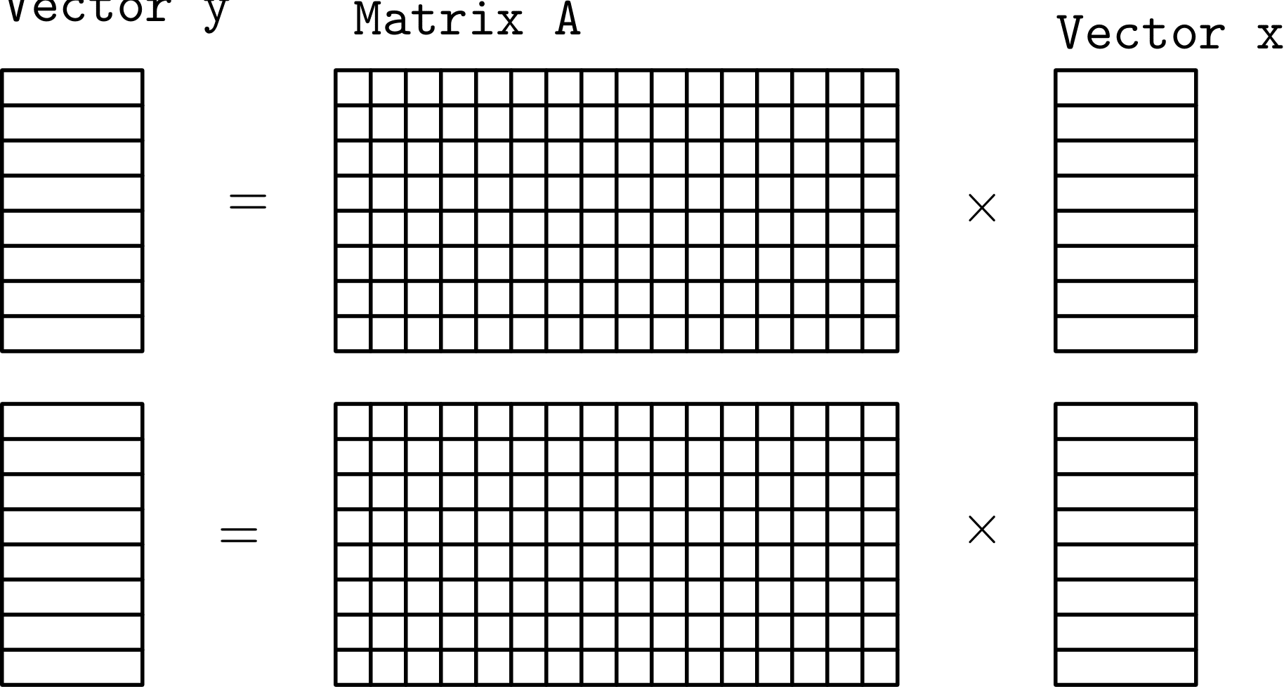
(For illustration purposes we represent the matrix as a dense matrix.) Conceptually this seems nice, but mathematically it is incorrect. Since we are partitioning the matrix so that each task has all of the columns of A we also need to be able to access all of the columns of x – so we can’t really partition x though we can partition y and we can partition A – row wise.

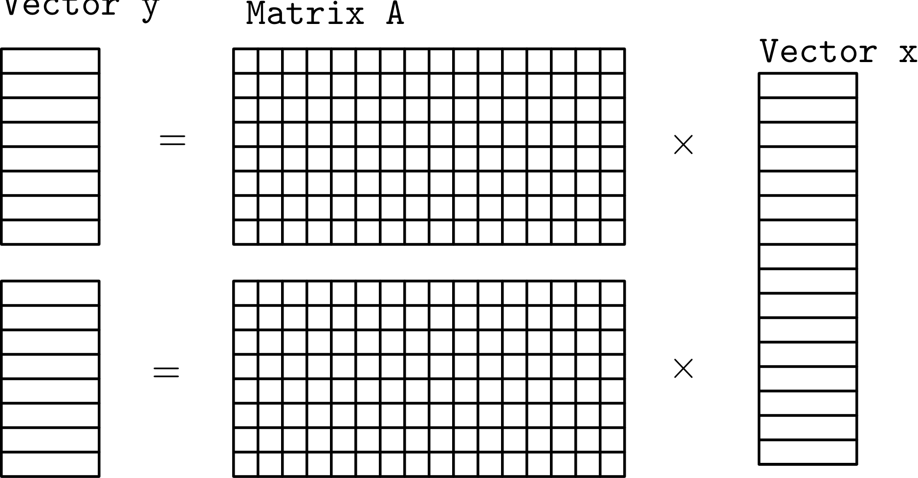
If we did want to split up x, we could partition A column wise but then each task has all of the rows of A so we can’t partition y.

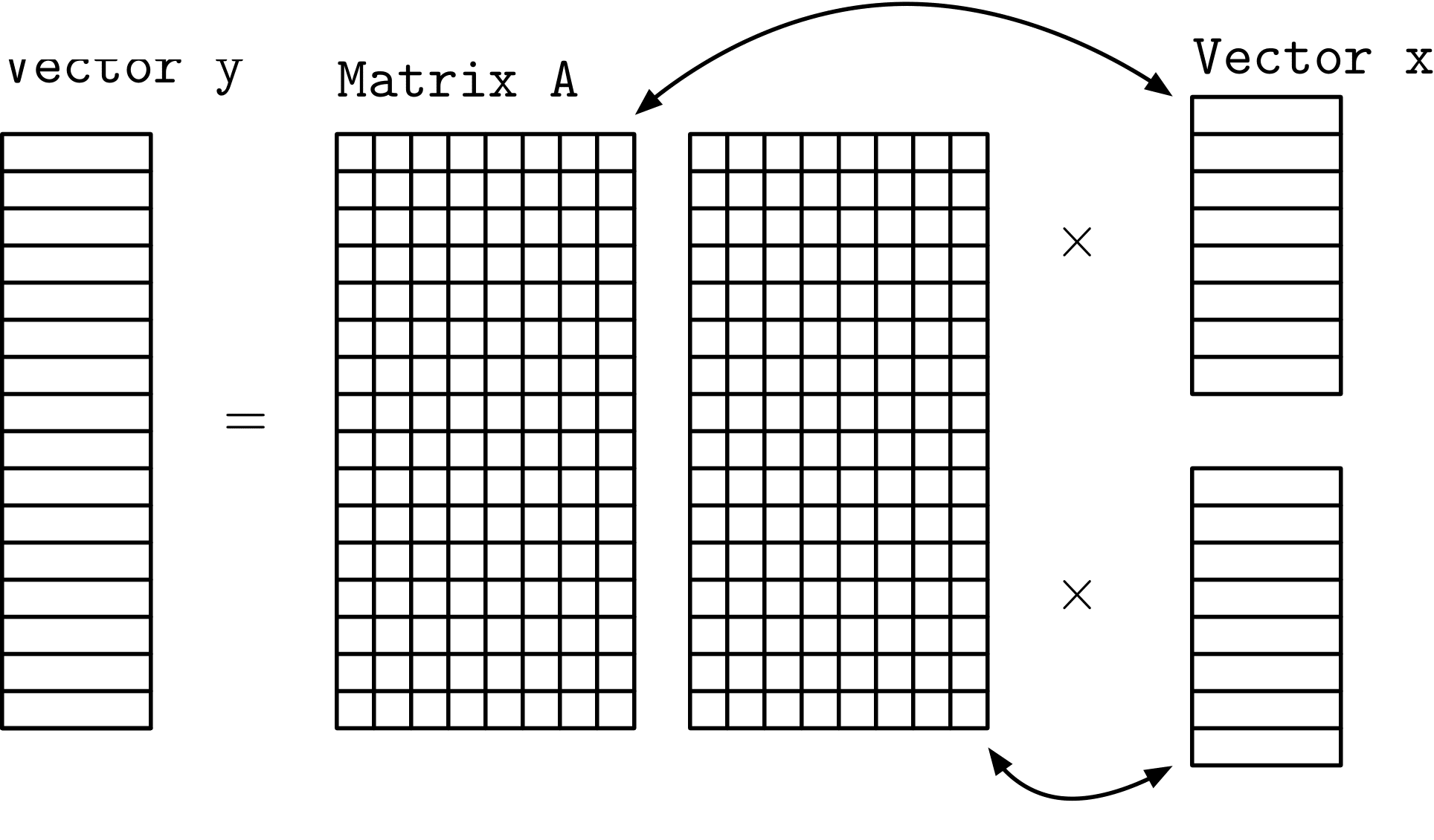
(Answer not required in Questions.rst but you should think about this.) What does this situation look like if we are computing the transpose product? If we partition A by rows and want to take the transpose product against x can we partition x or y? Similarly, if we partition A by columns can we partition x or y?

Accelerating PageRank¶

Your ps5 subdirectory contains a program pagerank.cpp. It takes as an argument a file specifying a graph (a set of connections), creates a right stochastic sparse matrix with that and then runs the pagerank algorithm. The program also takes optional flag arguments

$ ./pagerank.exe
Usage: ./pagerank.exe [-l label_file] [-a alpha] [-t tol] [-n num_threads] [-i max_iters] [-v N] input_file

The -l option specifies an auxiliary file that can contain label information for the entities being ranked (there is only one example I have with a label file), the -a option specifies the “alpha” parameter for the pagerank algorithm, -t specifies the convergence tolerance, -n specifies the number of threads to run with the program, -i specifies the maximum number of iterations to run of the pagerank algorithm, and -v specifies how many entries of the (ranked) output to print.

There are some small examples files in the ps5/data subdirectory:

$ ./pagerank.exe -l data/Erdos02_nodename.txt -v 10 data/Erdos02.mtx
# elapsed time [read]: 8 ms
Converged in 41 iterations
# elapsed time [pagerank]: 2 ms
0       0.000921655
1       0.00149955
2       0.000289607
3       0.00148465
4       0.000905182
5       0.00141333
6       0.000174406
7       0.00106162
8       0.000445909
9       0.000400393
# elapsed time [rank]: 0 ms
0       6926    0.0190492       ERDOS PAUL
1       502     0.0026224       ZAKS, SHMUEL
2       303     0.00259231      MCELIECE, ROBERT J.
3       444     0.00256273      STRAUS, ERNST GABOR*
4       261     0.00252477      KRANTZ, STEVEN GEORGE
5       391     0.00240435      SALAT, TIBOR
6       354     0.00239376      PREISS, DAVID
7       299     0.0023167       MAULDIN, R. DANIEL
8       231     0.00230076      JOO, ISTVAN*
9       474     0.00223145      TUZA, ZSOLT

This prints the time the program ran and since we had specified 10 to the -v option, it prints the first 10 values of the pagerank vector and then the entries corresponding to the 10 largest values. Since we had a label file in this case we also printed the associated labels. As expected, Paul Erdos is at the top.

The file Erdos02.mtx contains a co-authorship list of various authors. Running pagerank on that data doesn’t compute Erdos numbers, but it does tell us (maybe) who are the “important” authors in that network.

Erdos02.mtx is a very small network – 6927 authors and 8472 links and our C++ program computes its pagerank in just few milliseconds – hardly worth the trouble to accelerate. However, many problems of interest are much larger (such as the network of links in the world wide web).

Conundrum #2¶

Or is CSR::t_matvec the function we want to speed up?

Ideally, we would just add another argument to the call to mult in pagerank and invoke the parallel version. But getting high performance from an application involves creating the application so it functions efficiently as a whole. As the creator of the application, you get to (have to) make the decisions about what pieces to use for a particular situation.

In the case of pagerank.cpp I wrote this initially using the CSR sparse matrix format – that’s usually a reasonable default data structure to use. But, in pagerank we are not calling CSR::matvec rather we are calling CSR::t_matvec – which would be fine – for a purely sequential program. And now we want to parallelize it to improve the performance.

But, we have control over the entire application. We don’t need to simply dive down to the most expensive operation and parallelize that. We can also evaluate the application as a whole and think about some of the other decisions we made – and perhaps make different decisions that would let us accomplish the acceleration we want to more easily.

To be more specific. Above we noted that only two of the six “matrix vector” multiply variants were actually amenable to partition-based parallelization. Since mult is the kernel operation in pagerank, we should think about perhaps choosing an appropriate data structure so that we can take advantage of the opportunities for parallelization. And realize also we don’t have to call the transpose matrix product to compute the transposed product (we could send in the transposed matrix).

The second discussion I would like to see on Piazza is:

1. What are the two “matrix vector” operations that we could use?

2. How would we use the first in pagerank? I.e., what would we have to do differently in the rest of pagerank.cpp to use that first operation?

3. How would we use the second?

Answer these questions also in Questions.rst.

Implement one of the alternatives we discuss as a class.

For this problem – and this problem only – you may share small snippets of code on Piazza. It’s okay if everyone turns in the same two (or so) solutions – but everyone needs to actually put the code into the right place in their files and compile and run themselves. You should not need to change anything but the files pagerank.hpp and pagerank.cpp so snippets of shared code should be restricted to those files. Don’t reveal answers, for instance, from the sparse matrix-vector multiply implementations.

What is the largest graph you solved?