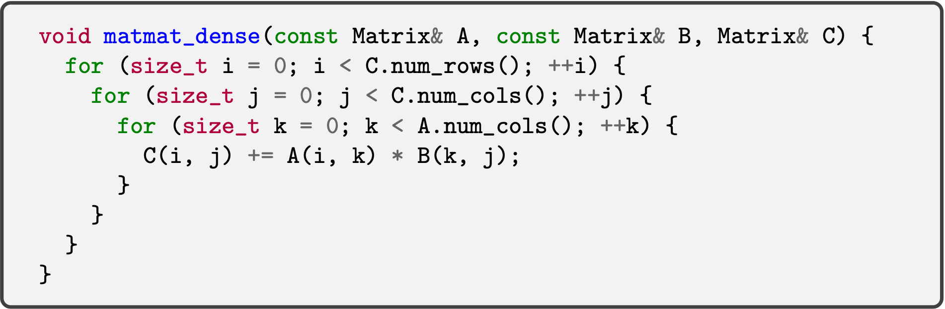
Lecture 8: Optimizing Dense Matrix-Matrix Product¶

The Roofline Model¶

By now you have probably noticed there are two things that come into play when trying to estimate the performance or the efficiency of a computation: how fast the arithmetic operations can be done – and how fast the data can be supplied to the arithmetic unit to do the operations. We know we can never compute faster than the maximum rate of the processor, but we also know we can’t compute faster than the memory subsystem can feed the processor. How do we know which bound to use and how do we use it?

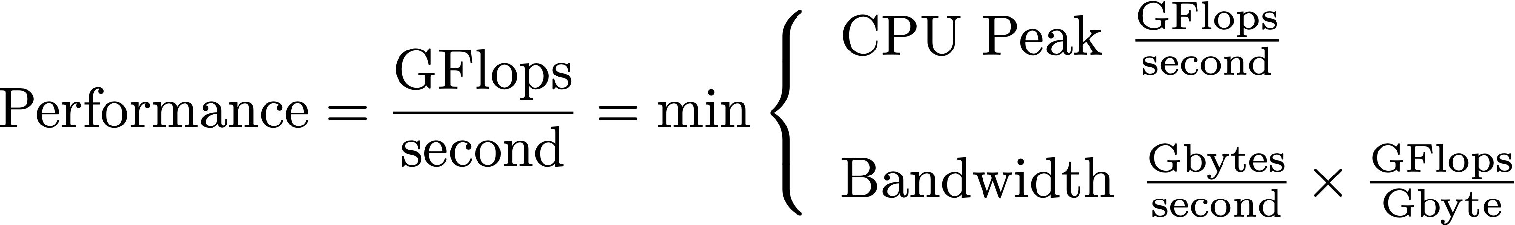
The roofline model was developed by computer scientists at UC Berkeley to address exactly this problem. The key insight in the roofline model is the notion of “arithmetic intensity” of a computation. That is, how many flops per byte are performed by the computation. The maximum performance measured in GFlops/sec is thus the maximum of the computing rate or the bandwidth times numerical intensity:

Peak performance and bandwidth thus give us two lines on a chart that plots GFlops/s vs numerical intensity. One line, CPU peak is independent of numeric intensity and so is horizontal. The other line is the ratio between GFlops/s and numerical intensity, i.e., bandwidth, which produces a sloped line on the chart.

We in fact have multiple lines of each kind to choose from. Max CPU performance depends on whether AVX instructions are being used, whether fused multiply-add is being used, for example. Bandwidth depends on where the data are in memory. Bandwidth to L1 caches is much higher than bandwidth to L2 cache, which is much higher than bandwidth to main memory. Each of these regimes deserve a line on the roofline model chart.

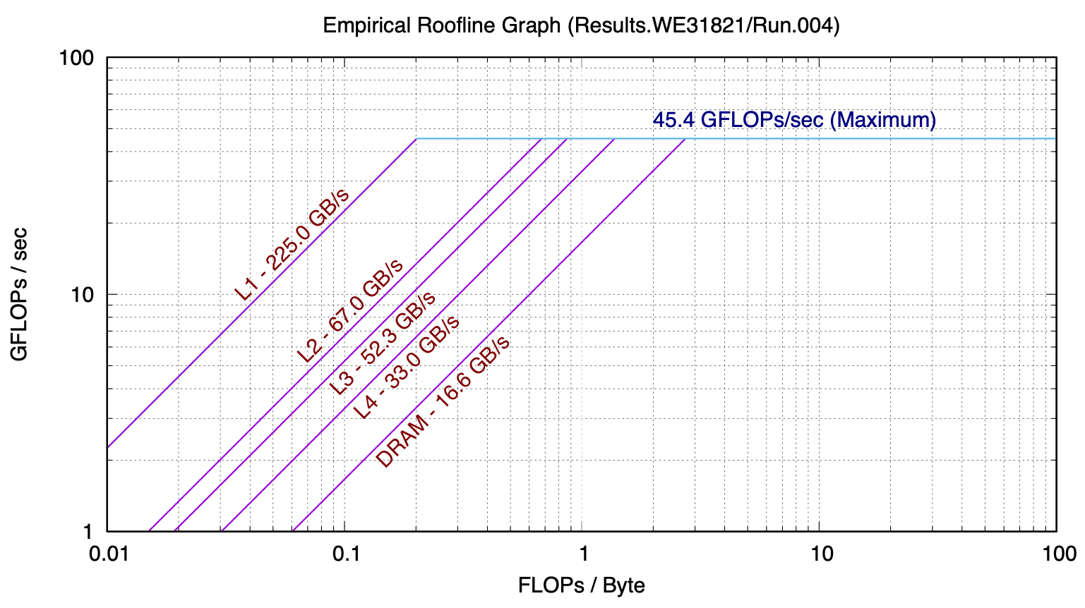
The following is a roofline model for a recent model MacBook Pro, gathered with Berkeley Lab’s Empirical Roofline Toolkit:

This model, while seemingly very simple, has strong predictive power.

Consider the case of the algorithm we have been studying – matrix-matrix product.

If we count the flops and bytes we see that the basic algorithm with no reuse has a numeric intensity of 1/12 flop/byte. We can use the ert chart to predict how many GFlops/second we would see from that. Let’s consider the case of a large problem, where, if there is no reuse the data would reside in main memory. Then we can see where the DRAM line intersects 1/12 on the x-axis – about 0.4 GFLOP/s

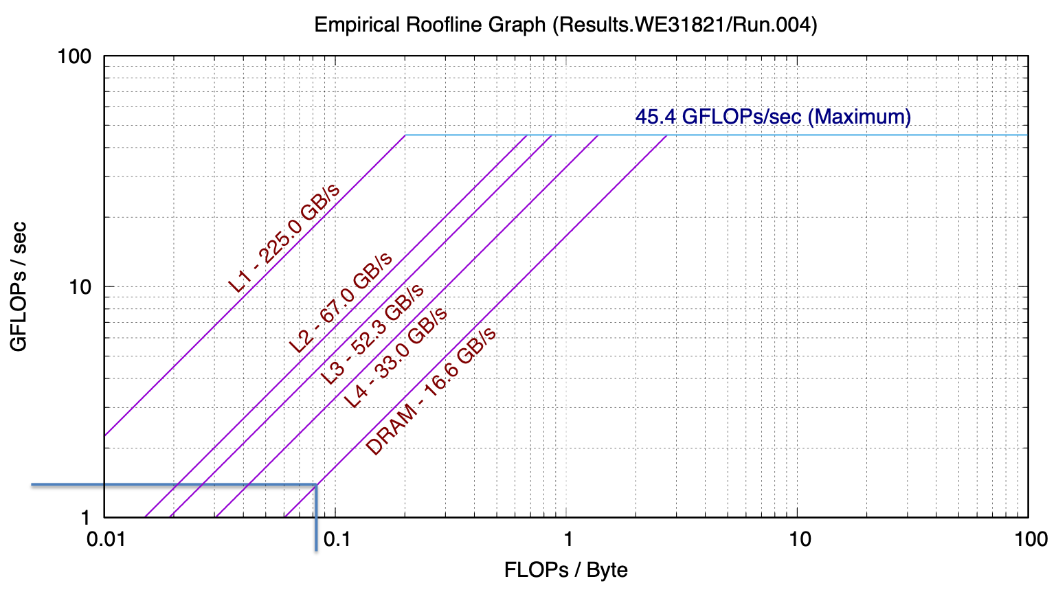
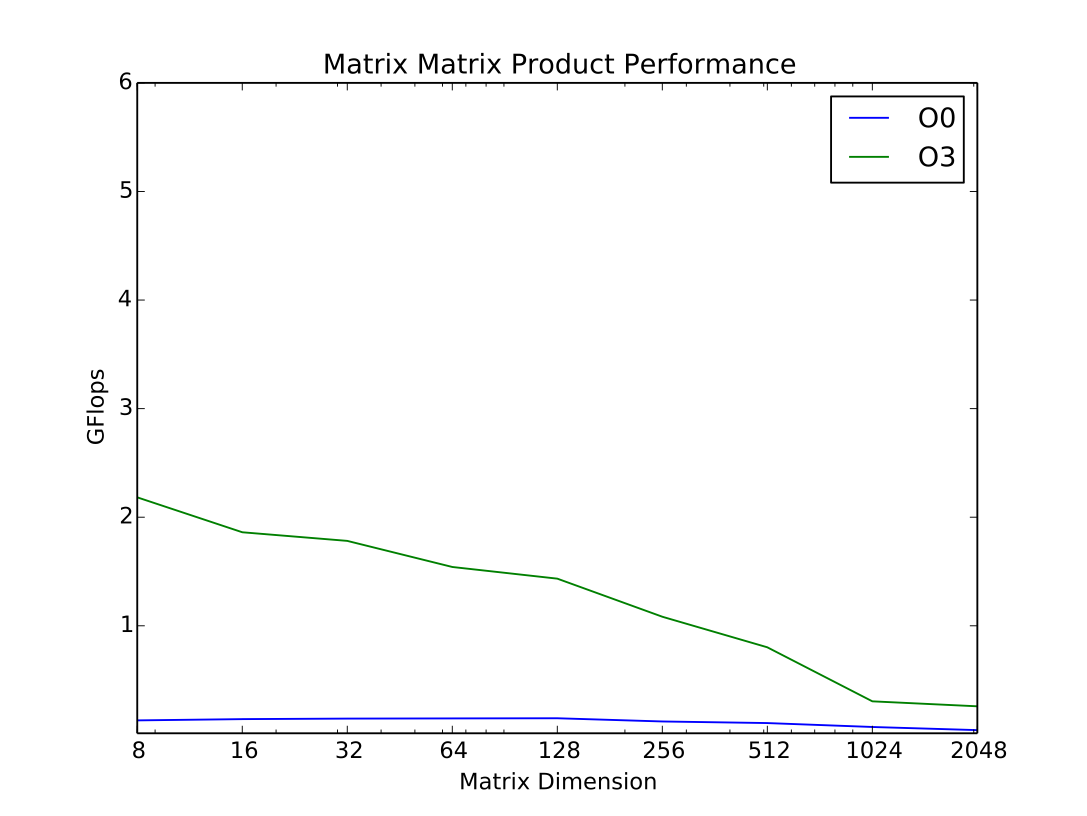
When we run matmat as is (without the reuse enhancing modifications), we see that for large problems we do in fact measure 0.4 GFlop/s.

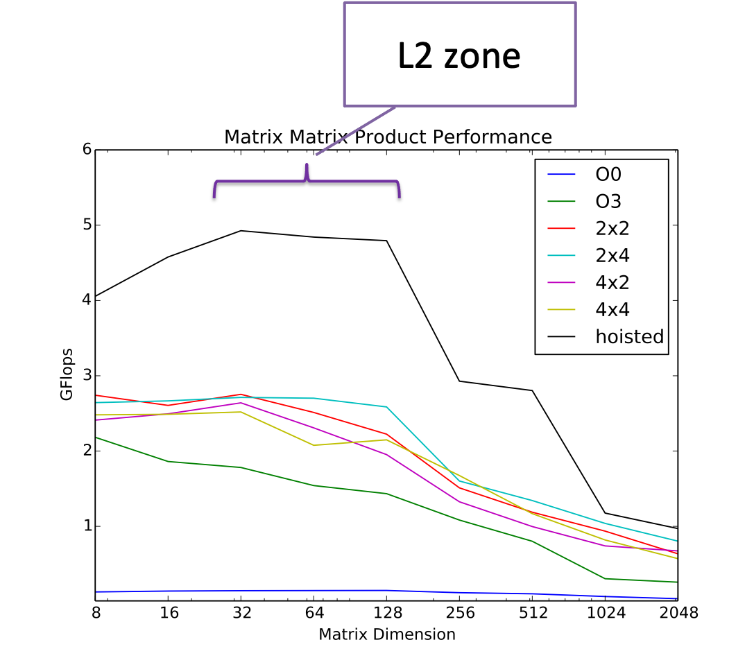
Let’s consider instead the case where we are making good use of cache and most of our problem is in L2 and we’ve applied some techniques for reuse. In that case, what we read off the chart is around 5 GFlop/s

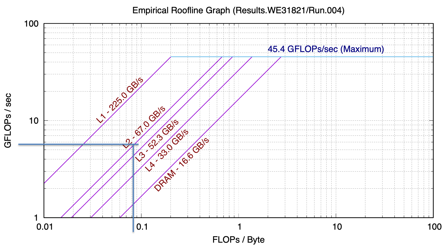
Looking at the actual measured performance, for problem sizes that fit in L2 cache, we see that we achieve approximately 5 GFlops/s: